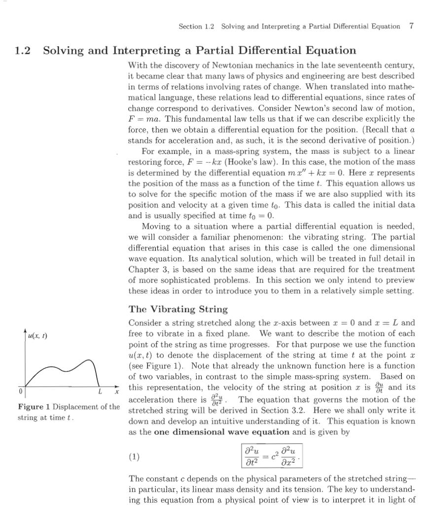
Section 1.2 Solving and Interpreting a Partial Differential Equation 7 1.2 Solving and Interpreting a Partial Differential Equation With the discovery of Newtonian mechanics in the late seventeenth century, it became clear that many laws of physics and engineering are best described in terms of relations involving rates of change.When translated into mathe- matical language,these relations lead to differential equations,since rates of change correspond to derivatives.Consider Newton's second law of motion, F=ma.This fundamental law tells us that if we can describe explicitly the force,then we obtain a differential equation for the position.(Recall that a stands for acceleration and,as such,it is the second derivative of position. For example,in a mass-spring system,the mass is subject to a linear restoring force,F=-kx(Hooke's law).In this case,the motion of the mass is determined by the differential equation mz"+k=0.Here z represents the position of the mass as a function of the time t.This equation allows us to solve for the specific motion of the mass if we are also supplied with its position and velocity at a given time to.This data is called the initial data and is usually specified at time to =0. Moving to a situation where a partial differential equation is needed, we will consider a familiar phenomenon:the vibrating string.The partial differential equation that arises in this case is called the one dimensional wave equation.Its analytical solution,which will be treated in full detail in Chapter 3,is based on the same ideas that are required for the treatment of more sophisticated problems.In this section we only intend to preview these ideas in order to introduce you to them in a relatively simple setting. The Vibrating String Consider a string stretched along the z-axis between x=0 and x=L and u(x,1) free to vibrate in a fixed plane.We want to describe the motion of each point of the string as time progresses.For that purpose we use the function u(x,t)to denote the displacement of the string at time t at the point x (see Figure 1).Note that already the unknown function here is a function of two variables,in contrast to the simple mass-spring system.Based on this representation,the velocity of the string at position isand its acceleration there is.The equation that governs the motion of the Figure 1 Displacement of the stretched string will be derived in Section 3.2.Here we shall only write it string at time t. down and develop an intuitive understanding of it.This equation is known as the one dimensional wave equation and is given by Bu (1) 282u 0t2 = 0x2 The constant c depends on the physical parameters of the stretched string- in particular,its linear mass density and its tension.The key to understand- ing this equation from a physical point of view is to interpret it in light of
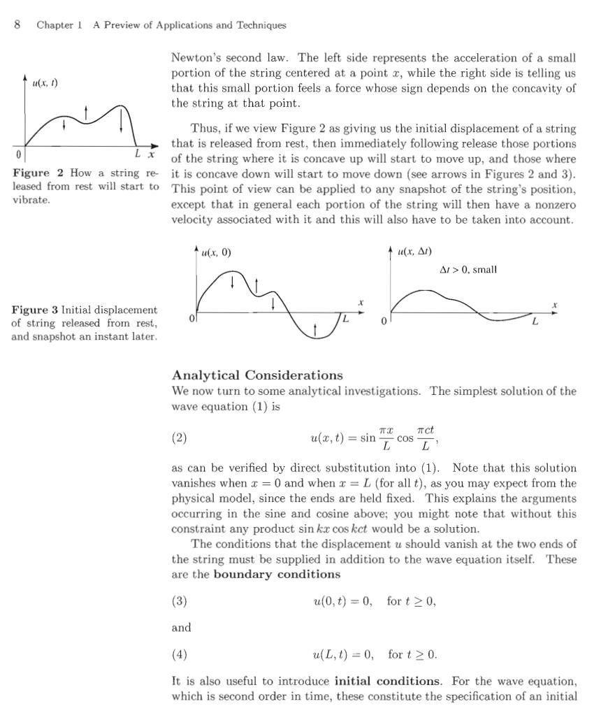
8 Chapter 1 A Preview of Applications and Techniques Newton's second law.The left side represents the acceleration of a small portion of the string centered at a point x,while the right side is telling us (f) that this small portion feels a force whose sign depends on the concavity of the string at that point. Thus,if we view Figure 2 as giving us the initial displacement of a string that is released from rest,then immediately following release those portions 0 of the string where it is concave up will start to move up,and those where Figure 2 How a string re-it is concave down will start to move down(see arrows in Figures 2 and 3). leased from rest will start to This point of view can be applied to any snapshot of the string's position, vibrate. except that in general each portion of the string will then have a nonzero velocity associated with it and this will also have to be taken into account. ↑(,0) ↑u(x,△) △/>0,small Figure 3 Initial displacement of string released from rest, and snapshot an instant later. Analytical Considerations We now turn to some analytical investigations.The simplest solution of the wave equation (1)is (2) mac xct u(z,t)=sin元cosD as can be verified by direct substitution into (1).Note that this solution vanishes when x =0 and when =L(for all t),as you may expect from the physical model,since the ends are held fixed.This explains the arguments occurring in the sine and cosine above;you might note that without this constraint any product sin ka cos kct would be a solution. The conditions that the displacement u should vanish at the two ends of the string must be supplied in addition to the wave equation itself.These are the boundary conditions (3) u(0,t)=0,fort≥0, and (4) u(L,t)=0,fort≥0 It is also useful to introduce initial conditions.For the wave equation, which is second order in time,these constitute the specification of an initial

Section 1.2 Solving and Interpreting a Partial Differential Equation 9 displacement and an initial velocity for some initial time to,henceforth taken as to =0: (5) u(x,0)=f(x),for0≤x≤L, Initial shape of the string and (x) (6) (红,0)=g,for0≤x≤L. The functions f(x)and g(z)represent arbitrary initial displacements and Initial velocity velocities along the string.You should imagine the string starting at time 8(x) t=0 with initial shape given by f(x)and initial velocity given by g(x)(see Figure 4). Let's look at the initial displacement and velocity of the solution (2) 0 L exhibited above.By setting t =0,we find the initial displacement to be Figure 4 Arbitrary initial displacement and velocity. u(z,0)=sin元 C for0≤x≤L. Similarly,by taking the partial derivative with respect to t,we obtain the initial velocity a(c,0)=0for0≤x≤h. O Thus (2)represents the solution where the string starts from rest with an initial displacement given by one arch of the sine function.There are many other similar solutions,but this one is surely the simplest.For example, you can verify that (7) RT ict u(z,t)=sin元sinT is also a solution to the wave equation (1)with boundary conditions(3)-(4). but now the initial displacement is 0 while the initial velocity is proportional to one arch of a sine.This corresponds to a string that is given a push starting from its rest position. The String in Slow Motion Consider the vibrating string as given by the solution (2).If you take snapshots of this string at various times,you will arrive at a sequence of pictures as shown in Figure 5(where L=1,c=1)
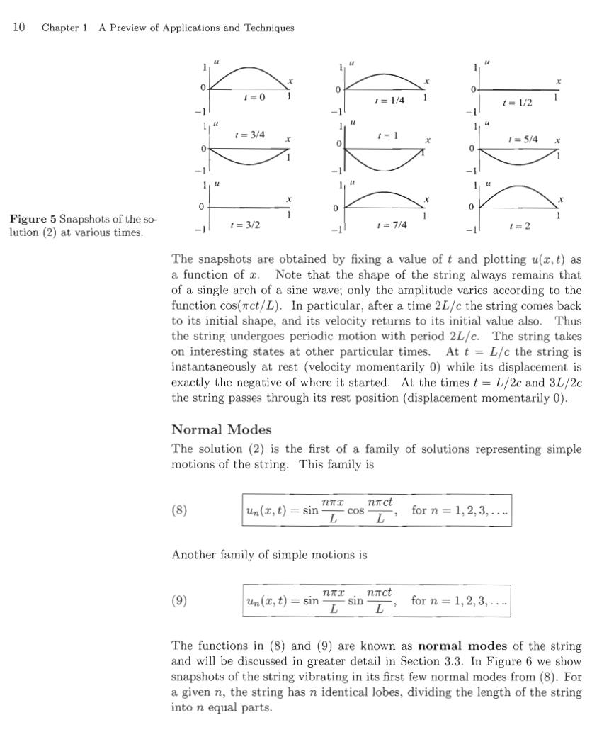
10 Chapter 1 A Preview of Applications and Techniques t=0 t=1/4 t=1/2 t=3/4 1=5/4 Figure 5 Snapshots of the so- 4=3/2 1=7/4 1=2 lution(2)at various times. The snapshots are obtained by fixing a value of t and plotting u(x,t)as a function of z.Note that the shape of the string always remains that of a single arch of a sine wave;only the amplitude varies according to the function cos(mct/L).In particular,after a time 2L/c the string comes back to its initial shape,and its velocity returns to its initial value also.Thus the string undergoes periodic motion with period 2L/c.The string takes on interesting states at other particular times.At t =L/c the string is instantaneously at rest (velocity momentarily 0)while its displacement is exactly the negative of where it started.At the times t=L/2c and 3L/2c the string passes through its rest position(displacement momentarily 0). Normal Modes The solution (2)is the first of a family of solutions representing simple motions of the string.This family is nπx (8) un(x,t)=sin nnct L, forn=1,2,3,..- Another family of simple motions is (9) 几Tx。 nict un(x,)=sin元sinD, forn=1,2,3,… The functions in (8)and (9)are known as normal modes of the string and will be discussed in greater detail in Section 3.3.In Figure 6 we show snapshots of the string vibrating in its first few normal modes from (8).For a given n,the string has n identical lobes,dividing the length of the string into n equal parts

Section 1.2 Solving and Interpreting a Partial Differential Equation 11 n=1 n=2 n=3 4=0 14 1=0 1s0 1=1/3 t=1/6 =1/9 0.5 0 1=2/3 1=1/3 1=2/9 t=1 -1 t=1/2 1=13 Figure 6 Normal modes from (8),for n =1,2,3 (with L 1 and c =1).Note that the higher modes oscillate more rapidly. Building Up More Complicated Motions: Superposition Principle and Fourier Series Thus far we have considered simple motions of the string.Surely the string can be set to vibrate in much more complicated ways.Can we describe all possible motions of the string?Before tackling this question,let's think of some examples of more complicated motions.Consider the following function built up by adding a number of scaled normal modes form (8): u(x,0) 2sin2mxcos2mt+3sin3mxcos3mt. 1 u(x,t)=sinπx cos mt- For simplicity,we have taken L=c=1.You should check that this is a 0.5 solution to (1)with c 1.At time t =0,the initial shape of the string is given by Figure 7 Initial shape of the string. u(,0)=sinsin2x+sin3ma, as illustrated in Figure 7.The velocity at time t,is given by Ou ()--sinsint+sin2mzsin2mt-sin 3m sin3t. Setting t =0,we see that the initial velocity is 0.Snapshots of the subse- quent motion can be obtained by plotting the function u as a function of x, for fixed values of t.The resulting graphs are shown in Figure 8. The process for building more complicated solutions by adding simpler ones is very important.This process is referred to formally as the superpo- sition principle and will be presented in its proper context in Section 3.1. This is the most important technique for constructing solutions to linear partial differential equations