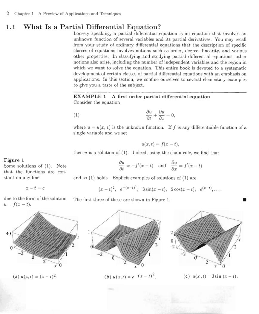
2 Chapter 1 A Preview of Applications and Techniques 1.1 What Is a Partial Differential Equation? Loosely speaking,a partial differential equation is an equation that involves an unknown function of several variables and its partial derivatives.You may recall from your study of ordinary differential equations that the description of specific classes of equations involves notions such as order,degree,linearity,and various other properties.In classifying and studying partial differential equations,other notions also arise,including the number of independent variables and the region in which we want to solve the equation.This entire book is devoted to a systematic development of certain classes of partial differential equations with an emphasis on applications.In this section,we confine ourselves to several elementary examples to give you a taste of the subject. EXAMPLE 1 A first order partial differential equation Consider the equation (1)) Ouou +证 =0, where u=u(x,t)is the unknown function.If f is any differentiable function of a single variable and we set u(x,t)=f(x-t), then u is a solution of(1).Indeed,using the chain rule,we find that Figure 1 Some solutions of (1).Note 欲=-fe-0and Ou Ox =红-) that the functions are con- stant on any line and so (1)holds.Explicit examples of solutions of (1)are x-t=c (z-t2,e-x-°,3sin(x-t),2cos(红-t,ea-),… due to the form of the solution The first three of these are shown in Figure 1. u=f(x-t). 40 0 0 (a)u(x,f)=(x-t)2 (b)u(x,)=e-(x-)2 (c)u(x.t)=3sin (x-1)
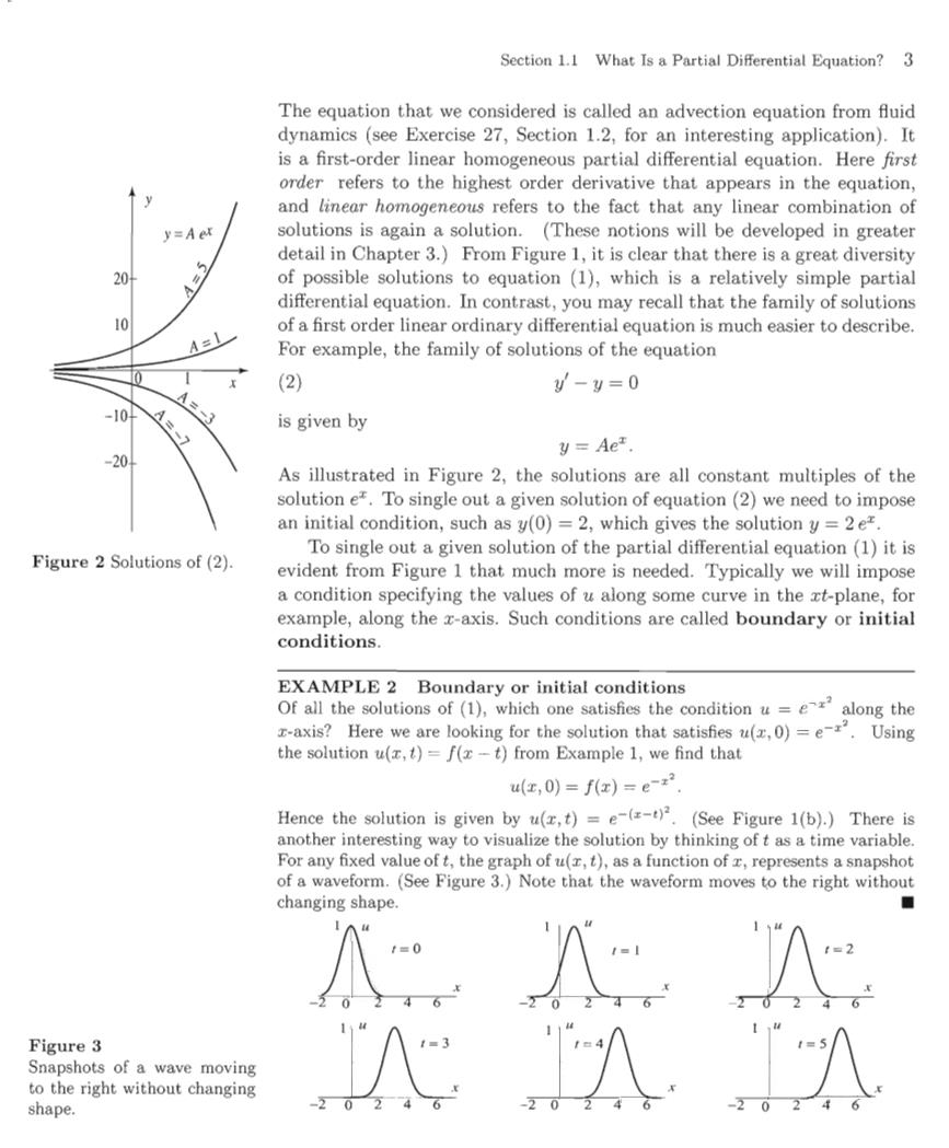
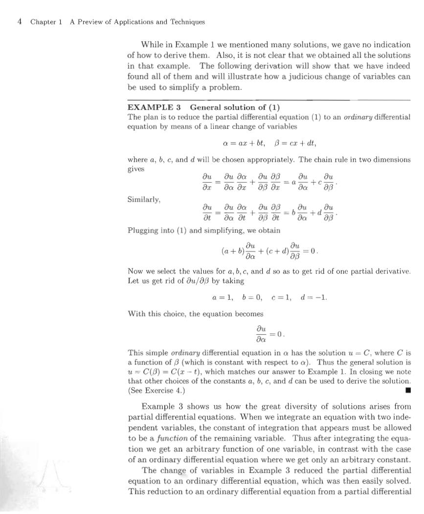
Section 1.1 What Is a Partial Differential Equation?3 The equation that we considered is called an advection equation from fluid dynamics (see Exercise 27,Section 1.2,for an interesting application).It is a first-order linear homogeneous partial differential equation.Here first order refers to the highest order derivative that appears in the equation, and linear homogeneous refers to the fact that any linear combination of y=Aer solutions is again a solution.(These notions will be developed in greater detail in Chapter 3.)From Figure 1,it is clear that there is a great diversity 20- of possible solutions to equation (1),which is a relatively simple partial differential equation.In contrast,you may recall that the family of solutions 10 of a first order linear ordinary differential equation is much easier to describe. A=1 For example,the family of solutions of the equation (2) y-y=0 is given by y=Aet. As illustrated in Figure 2,the solutions are all constant multiples of the solution e.To single out a given solution of equation(2)we need to impose an initial condition,such as y(0)=2,which gives the solution y=2e=. To single out a given solution of the partial differential equation(1)it is Figure 2 Solutions of(2). evident from Figure 1 that much more is needed.Typically we will impose a condition specifying the values of u along some curve in the xt-plane,for example,along the x-axis.Such conditions are called boundary or initial conditions. EXAMPLE 2 Boundary or initial conditions Of all the solutions of(1),which one satisfies the condition u=ealong the r-axis?Here we are looking for the solution that satisfies u(,0)=e-.Using the solution u(x,t)=f(x-t)from Example 1,we find that u(z,0)=fx)=e-x2 Hence the solution is given by u(,t)=e-(-).(See Figure 1(b).)There is another interesting way to visualize the solution by thinking of t as a time variable. For any fixed value of t,the graph of u(r,t),as a function of z,represents a snapshot of a waveform.(See Figure 3.)Note that the waveform moves to the right without changing shape ■ 八八 Figure 3 Snapshots of a wave moving to the right without changing shape
4 Chapter 1 A Preview of Applications and Techniques While in Example 1 we mentioned many solutions,we gave no indication of how to derive them.Also,it is not clear that we obtained all the solutions in that example.The following derivation will show that we have indeed found all of them and will illustrate how a judicious change of variables can be used to simplify a problem. EXAMPLE 3 General solution of(1) The plan is to reduce the partial differential equation(1)to an ordinary differential equation by means of a linear change of variables a=ax+bt,B=cx+dt, where a,b,c,and d will be chosen appropriately.The chain rule in two dimensions gives Ou ou da Ou 8B ouOu =aa0a证+0丽0证 =a- 8x +ca丽 a Similarly, Ou Ou Da 0ua3,0u. Ou OL=aa aa 8B at =6 +d 8B Plugging into(1)and simplifying,we obtain (a+b)Da Ou +(c+d) =0. Now we select the values for a,b,c,and d so as to get rid of one partial derivative. Let us get rid of ou/03 by taking a=1,b=0,c=1,d=-1. With this choice,the equation becomes ou =0. Ba This simple ordinary differential equation in a has the solution u =C,where C is a function of B(which is constant with respect to a).Thus the general solution is u=C(B)=C(-t),which matches our answer to Example 1.In closing we note that other choices of the constants a,b,c,and d can be used to derive the solution. (See Exercise 4.) ■ Example 3 shows us how the great diversity of solutions arises from partial differential equations.When we integrate an equation with two inde- pendent variables,the constant of integration that appears must be allowed to be a function of the remaining variable.Thus after integrating the equa- tion we get an arbitrary function of one variable,in contrast with the case of an ordinary differential equation where we get only an arbitrary constant. The change of variables in Example 3 reduced the partial differential equation to an ordinary differential equation,which was then easily solved. This reduction to an ordinary differential equation from a partial differential
Section 1.1 What Is a Partial Differential Equation?5 equation is a recurring theme throughout the book.(See Exercise 10 for another illustration. Exercises 1.1 1.Suppose that u1 and u2 are solutions of (1).Show that ciu+cau2 is also a solution,where ci and c2 are constants.(This shows that (1)is a linear equation.) 2.(a)Which solution of(1)is equal to re-on the x-axis? (b)Plot the solution asa function ofand,and describe the image of the-axis. 3.(a)Find the solution of (1)that is equal to t on the t-axis. (b)Plot the solution asa function ofandt,and describe the image of thet-axis. 4.Refer to Example 3 and solve (1)using a 1,b=1,c=1,d=-1. In Erercises 5-8,derive the general solution of the given equation by using an appropriate change of variables,as we did in Erample 3. 5.0-船=0. 6.2器+3器=0. 7,號-2器=2. 8.a8光+b8=u, a,b≠0. 9.(a)Find the solution in Exercise 5 that is equal to along the axis (b)Plot the graph of the solution as a function of z and t. (c)In what direction is the waveform moving as t increases? The method of characteristic curves This method allows you to solve first order,linear partial differential equations with nonconstant coefficients of the form (3) O 0u=0, 正+红》 where p(,y)is a function of z and y.We begin by reviewing two important concepts from calculus of several variables and ordinary differential equations. Suppose that v =(v1,v2)is a unit vector and u(,y)is a function of two variables.The directional derivative of u (in the direction of v)at the point (o,y0)is given by Ou ou ”20b)+ (x0,0) The directional derivative measures the rate of change of u at the point (zo,yo)as we move in the direction of v.Consequently,if (a,b)is any nonzero vector,then the relation Ou ,ou a 左+b而 =0 states that u is not changing in the direction of (a,b). Moving to ordinary differential equations,consider the equation (4) dy dx =px,)

6 Chapter 1 A Preview of Applications and Techniques and think of the solutions of (4)as curves in the xy-plane.Equation(4)is telling us that the slope of the tangent line to a solution curve at the point (zo,yo)is equal to p(xo,yo),or that the solution curve at the point(zo,yo)is changing in the direction of the vector (1,p(xo,y0)).If we plot the vectors (1,p(,y))for many points (y), we obtain the direction field for the differential equation(4).The direction field is very important,since it gives us a quick way for visualizing the qualitative behavior of the solutions of(4).In particular,we can trace a solution curve through a point (,y)by constantly moving in the direction of the vector field(1,p(,)). We are now ready to present the method of characteristic curves.Going back to(3),this equation is telling us that,at any point (,y),the directional derivative of u in the direction of the vector(1,p(,y))is 0.Hence u(,y)remains constant if from the point (z,y)we move in the direction of vector (1,p(,y)).But the vector (1,p(x,y))determines the direction field for (4).Consequently,u is constant on the solution curves of(4).These curves are called the characteristic curves of(3) (see Figure 4 for the case p(,y)=x,treated below).For convenience,let us write the solutions of(4)(the characteristic curves)in the form (x,y)=C, where C is arbitrary.Since u is constant on each such curve,the values of u depend only on C.Thus u(x,y)=f(C),where f is an arbitrary function,or u(x,)=f((x,), which yields the solution of(3). As an illustration,let us solve the equation OuOu =0. 0 + We have p()=z.Solving=,we find the characteristic curvesy=C, or y-x2=C.Hence (y)=y-r2,and the general solution of the partial differential equation is u(z,y)=f((,y)),where f is an arbitrary function.The Figure 4 Direction field for validity of this solution can be checked directly by plugging it back into the equation. =z and the characteristic It is worth noting that in solving the partial differential equation (3)by the curves y2=C. method of characteristic curves,all we had to do is solve the ordinary differential equation (4).Thus,the method of characteristic curves is yet another method that reduces a partial differential equation to an ordinary differential equation. 10.Consider the equation0,whereare nonzero constants. (a)What is the equation saying about the directional derivative of u? (b)Determine the characteristic curves. (c)Solve the equation using the method of characteristic curves. In Exercises 11-14,(a)solve the given equation by the method of characteristic curves,and (b)check your answer by plugging it back into the equation. 11.器+x器=0. 12.x器+y踹=0. 13.器+sinx踹=0. 14.e28器+x器=0