透 3 Analyzing Data Objectives In this chapter,you: Display and interpret descriptive statistics,page 3-2 Perform and interpret a one-way ANOVA,page 3-4 Display and interpret built-in graphs,page 34 Access the StatGuide,page 3-8 Use the Project Manager,page 3-10 Overview The field of statistics provides principles and methodologies for collecting, summarizing,analyzing,and interpreting data,and for drawing conclusions from analysis results.Statistics can be used to describe data and to make inferences,both of which can guide decisions and improve processes and products MINTTAB provides: Many statistical methods organized by category,such as regression,ANOVA, quality tools,and time series Built-in graphs to help you understand the data and validate results The ability to display and store statistics and diagnostic measures This chapter introduces MINTTAB's statistical commands,built-in graphs,StatGuide, and Project Manager.You want to assess the number of late and back orders,and test whether the difference in delivery time among the three shipping centers is statistically significant. 暇 For more information on MINITAB's statistical features,go to Stat menu in the MINITAB Help index. Meet MINITAB 3-1
Meet MINITAB 3-1 3 Analyzing Data Objectives In this chapter, you: ■ Display and interpret descriptive statistics, page 3-2 ■ Perform and interpret a one-way ANOVA, page 3-4 ■ Display and interpret built-in graphs, page 3-4 ■ Access the StatGuide, page 3-8 ■ Use the Project Manager, page 3-10 Overview The field of statistics provides principles and methodologies for collecting, summarizing, analyzing, and interpreting data, and for drawing conclusions from analysis results. Statistics can be used to describe data and to make inferences, both of which can guide decisions and improve processes and products. MINITAB provides: ■ Many statistical methods organized by category, such as regression, ANOVA, quality tools, and time series ■ Built-in graphs to help you understand the data and validate results ■ The ability to display and store statistics and diagnostic measures This chapter introduces MINITAB’s statistical commands, built-in graphs, StatGuide, and Project Manager. You want to assess the number of late and back orders, and test whether the difference in delivery time among the three shipping centers is statistically significant. For more information on MINITAB’S statistical features, go to Stat menu in the MINITAB Help index
Chapter 3 Displaying Descriptive Statistics Displaying Descriptive Statistics Descriptive statistics summarize and describe the prominent features of data. Use Display Descriptive Statistics to find out how many book orders were delivered on time,how many were late,and the number that were initially back ordered for each shipping center. Display 1 If continuing from the previous chapter,choose File >New,then choose descriptive Minitab Project.Click OK.Otherwise,just start MINITAB. statistics 2 Choose File Open Worksheet. 3 Double-click Meet MINITAB,then choose SHIPPINGDATA.MTW.Click Open.This worksheet is the same one you used in Chapter 2,Graphing Data. 4 Choose Stat Basic Statistics Dapin Descrperve Staities Display Descriptive Statistics. farishle图 5 In Variables,enter Days. 6 In By variables(optional),enter Center y variables loptiona啡 Status. For most MINTTAB commands,you only need to complete the main dialog box to execute the command.But,you can often use subdialog boxes to modify the Statistice Graphs analysis or display additional output, like graphs. Help g☐cal 7 Click Statistics. 8 Uncheck First quartile, E Median,Third quartile,N nonmissing,and N missing. 9 Check N total. percen 10 Click OK in each dialog box. Bieet quartile 厂5am0tsW*e5 DSikmw OK Csscel Changes made in the Statistics subdialog box affect the current session only.To change the default settings for future sessions,use Tools>Options>Individual Commands>Display Descriptive Statistics.When you open the Statistics subdialog box again,it reflects your preferences. 3-2 Meet MINITAB
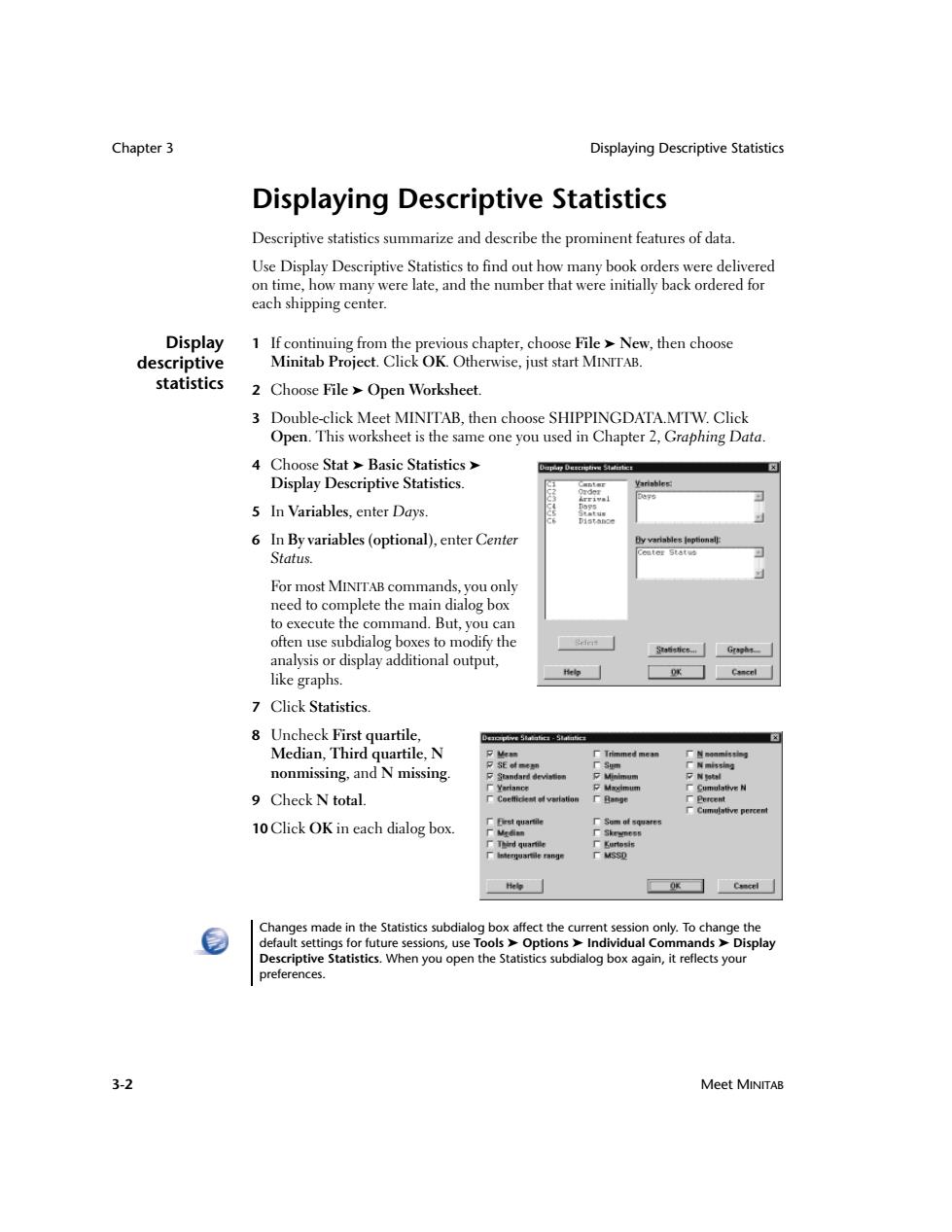
Chapter 3 Displaying Descriptive Statistics 3-2 Meet MINITAB Displaying Descriptive Statistics Descriptive statistics summarize and describe the prominent features of data. Use Display Descriptive Statistics to find out how many book orders were delivered on time, how many were late, and the number that were initially back ordered for each shipping center. Display descriptive statistics 1 If continuing from the previous chapter, choose File ➤ New, then choose Minitab Project. Click OK. Otherwise, just start MINITAB. 2 Choose File ➤ Open Worksheet. 3 Double-click Meet MINITAB, then choose SHIPPINGDATA.MTW. Click Open. This worksheet is the same one you used in Chapter 2, Graphing Data. 4 Choose Stat ➤ Basic Statistics ➤ Display Descriptive Statistics. 5 In Variables, enter Days. 6 In By variables (optional), enter Center Status. For most MINITAB commands, you only need to complete the main dialog box to execute the command. But, you can often use subdialog boxes to modify the analysis or display additional output, like graphs. 7 Click Statistics. 8 Uncheck First quartile, Median, Third quartile, N nonmissing, and N missing. 9 Check N total. 10 Click OK in each dialog box. Changes made in the Statistics subdialog box affect the current session only. To change the default settings for future sessions, use Tools ➤ Options ➤ Individual Commands ➤ Display Descriptive Statistics. When you open the Statistics subdialog box again, it reflects your preferences
Displaying Descriptive Statistics Analyzing Data Session Descriptive Statistics:Days window output Results for Center Central Total Variable Status Count Mean SE Mean StDev Minimum Maximum Days Back order 6 ★ ★ Late 66.431 0.1570.385 6.078 7.070 On time 933.826 0.1191.149 1.267 5.983 Results for Center Eastern Total Variable Status Count Mean SE Mean StDev Minimum Maximum Days Back order 8 Late 96.678 0.1800.541 6.254 7.748 On time 924.234 0.1121.077 1.860 5.953 Results for Center =Western Total Variable Status Count Mean SE Mean StDev Minimum Maximum Days Back order 3 On time 1022.981 0.1081.0900.871 5.681 The Session window displays text output,which you can edit,add to the ReportPad,and print. The ReportPad is discussed in Chapter 7,Generating a Report. Interpret The Session window presents each center's results separately.Within each center, results you can find the number of back,late,and on-time orders in the Total Count column The Eastern shipping center has the most back orders(8)and late orders(9). The Central shipping center has the next greatest number of back orders(6)and late orders (6). The Western shipping center has the smallest number of back orders(3)and no late orders. You can also review the Session window output for the mean,standard error of the mean,standard deviation,minimum,and maximum of order status for each center. These statistics are not given for back orders because no delivery information exists for these orders. Meet MINITAB 3-3
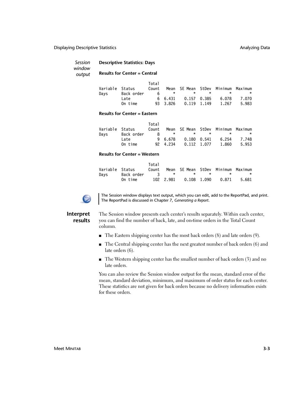
Displaying Descriptive Statistics Analyzing Data Meet MINITAB 3-3 Session window output Descriptive Statistics: Days Results for Center = Central Total Variable Status Count Mean SE Mean StDev Minimum Maximum Days Back order 6 * * * * * Late 6 6.431 0.157 0.385 6.078 7.070 On time 93 3.826 0.119 1.149 1.267 5.983 Results for Center = Eastern Total Variable Status Count Mean SE Mean StDev Minimum Maximum Days Back order 8 * * * * * Late 9 6.678 0.180 0.541 6.254 7.748 On time 92 4.234 0.112 1.077 1.860 5.953 Results for Center = Western Total Variable Status Count Mean SE Mean StDev Minimum Maximum Days Back order 3 * * * * * On time 102 2.981 0.108 1.090 0.871 5.681 Interpret results The Session window presents each center’s results separately. Within each center, you can find the number of back, late, and on-time orders in the Total Count column. ■ The Eastern shipping center has the most back orders (8) and late orders (9). ■ The Central shipping center has the next greatest number of back orders (6) and late orders (6). ■ The Western shipping center has the smallest number of back orders (3) and no late orders. You can also review the Session window output for the mean, standard error of the mean, standard deviation, minimum, and maximum of order status for each center. These statistics are not given for back orders because no delivery information exists for these orders. The Session window displays text output, which you can edit, add to the ReportPad, and print. The ReportPad is discussed in Chapter 7, Generating a Report
Chapter 3 Performing an ANOVA Performing an ANOVA One of the most commonly used methods in statistical decisions is hypothesis testing.MINITAB offers many hypothesis testing options,including t-tests and analysis of variance.Generally,a hypothesis test assumes an initial claim to be true,then tests this claim using sample data. Hypothesis tests include two hypotheses:the null hypothesis(denoted by Ho)and the alternative hypothesis(denoted by H).The null hypothesis is the initial claim and is often specified using previous research or common knowledge.The alternative hypothesis is what you may believe to be true. Based on the graphical analysis you performed in the previous chapter and the descriptive analysis above,you suspect that difference in the average number of delivery days(response)across shipping centers(factor)is statistically significant.To verify this,perform a one-way ANOVA,which tests the equality of two or more means categorized by a single factor.Also,conduct a Tukey's multiple comparison test to see which shipping center means are different. Perform an 1 Choose Stat ANOVA One-Way. Den.ay Anslyes n Vaiance ANOVA 2 In Response,enter Days.In Factor,enter tF Ae5 ponee:D保形 Center. In many dialog boxes for statistical Sinre tr移duas 厂Store ta: commands,you can choose frequently used or required options.Use the subdialog box buttons to choose other options. 3 Click Comparisons. 4 Check Tukey's,family error rate,then 女Iky family err rate click OK. 厂's.individual aror ra 厂、-s4多=ygr 厂eMC8.lamily erur rate Lemnestis beat 3-4 Meet MINITAB
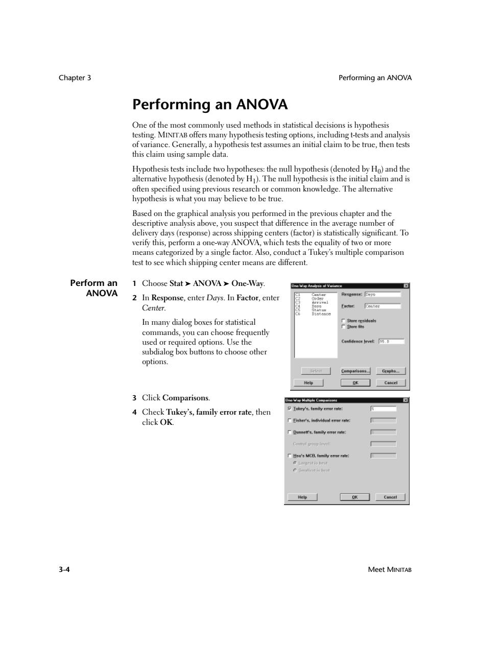
Chapter 3 Performing an ANOVA 3-4 Meet MINITAB Performing an ANOVA One of the most commonly used methods in statistical decisions is hypothesis testing. MINITAB offers many hypothesis testing options, including t-tests and analysis of variance. Generally, a hypothesis test assumes an initial claim to be true, then tests this claim using sample data. Hypothesis tests include two hypotheses: the null hypothesis (denoted by H0) and the alternative hypothesis (denoted by H1). The null hypothesis is the initial claim and is often specified using previous research or common knowledge. The alternative hypothesis is what you may believe to be true. Based on the graphical analysis you performed in the previous chapter and the descriptive analysis above, you suspect that difference in the average number of delivery days (response) across shipping centers (factor) is statistically significant. To verify this, perform a one-way ANOVA, which tests the equality of two or more means categorized by a single factor. Also, conduct a Tukey’s multiple comparison test to see which shipping center means are different. Perform an ANOVA 1 Choose Stat ➤ ANOVA ➤ One-Way. 2 In Response, enter Days. In Factor, enter Center. In many dialog boxes for statistical commands, you can choose frequently used or required options. Use the subdialog box buttons to choose other options. 3 Click Comparisons. 4 Check Tukey’s, family error rate, then click OK
Performing an ANOVA Analyzing Data 5 Click Graphs. For many statistical commands, Pexgilets of datn MINITAB includes built-in graphs that help you interpret Reaidual Plots IndMidual ploty the results and assess the validity of statistical assumptions. 厂ed时ysi倒 6 Check Individual value plot Four in ane and Boxplots of data. 7 Under Residual Plots,choose Four in one 冰☐ 8 Click OK in each dialog box. Session One-way ANOVA:Days versus Center window output Source DF SS MS Center 2114.6357.32 39.190.000 Error 299437.281.46 Total 301 551.92 S=1.209 R-Sq=20.77% R-Sq(adj)=20.24% Individual 95%CIs For Mean Based on Pooled StDev Level Mean StDev ------ Central 993.984 1.280 (----*--) Eastern 101 4.4521.252 (---*----】 Western 1022.981 1.090 (---*---) -----+- -+ ---+- ----+--- 3.00 3.50 4.00 4.50 Pooled StDev 1.209 Tukey 95%Simultaneous Confidence Intervals All Pairwise Comparisons among Levels of Center Individual confidence level 98.01% Center Central subtracted from: Center Lower Center Upper Eastern 0.068 0.4680.868 (--*-) Western -1.402 -1.003-0.603 (---*---)】 -1.0 0.0 1.0 2.0 Meet MINITAB 3-5
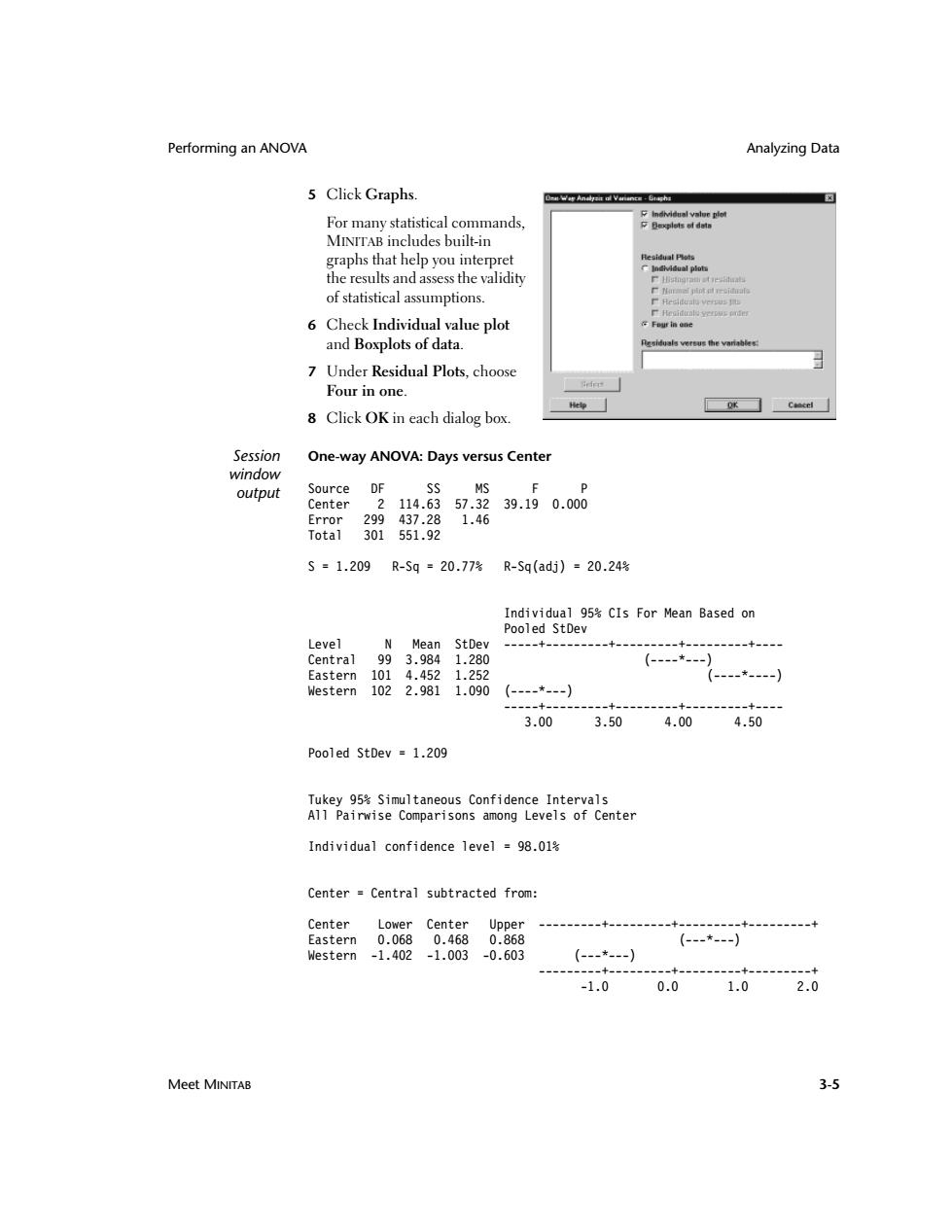
Performing an ANOVA Analyzing Data Meet MINITAB 3-5 5 Click Graphs. For many statistical commands, MINITAB includes built-in graphs that help you interpret the results and assess the validity of statistical assumptions. 6 Check Individual value plot and Boxplots of data. 7 Under Residual Plots, choose Four in one. 8 Click OK in each dialog box. Session window output One-way ANOVA: Days versus Center Source DF SS MS F P Center 2 114.63 57.32 39.19 0.000 Error 299 437.28 1.46 Total 301 551.92 S = 1.209 R-Sq = 20.77% R-Sq(adj) = 20.24% Individual 95% CIs For Mean Based on Pooled StDev Level N Mean StDev -----+---------+---------+---------+---- Central 99 3.984 1.280 (----*---) Eastern 101 4.452 1.252 (----*----) Western 102 2.981 1.090 (----*---) -----+---------+---------+---------+---- 3.00 3.50 4.00 4.50 Pooled StDev = 1.209 Tukey 95% Simultaneous Confidence Intervals All Pairwise Comparisons among Levels of Center Individual confidence level = 98.01% Center = Central subtracted from: Center Lower Center Upper ---------+---------+---------+---------+ Eastern 0.068 0.468 0.868 (---*---) Western -1.402 -1.003 -0.603 (---*---) ---------+---------+---------+---------+ -1.0 0.0 1.0 2.0