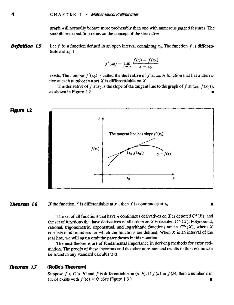
4 C HA PT E R 1.Mathematical Prellminaries graph will normally behave more predictably than one with numerous jagged features.The smoothness condition relies on the concept of the derivative. Definitlon 1.5 Let f be a function defined in an open interval containing xo.The function f is differen- tiable at xo if ')) )x-x0 exists.The mumber f'(xo)is called the derivative of f at xo.A function that has a deriva The der ative as shown in Figure t.2. Flgure 1.2 y The tangent line has slope f'(x fxo)十 xof6xo》 y=f(r) Theorem 1.6 If the function f is differentiable at xo.then f is continuous at xo. ◆ The set of all functions that haven continuous derivatives onXis denoted (X).and the set of functions that have derivatives of all orders on X is denoted c().Polynomial rational,trigonometric,exponential,and logarithmic functions are in C(X),where X consists of all numbers for which the functions are defined.When X is an interval of the real line,we will again omit the parentheses in this notation. The next theorems are of fundamental importance in deriving methods for error esti- matio proofs of these thorems and the oherrntin thisctioncan standard calculus text. Theorem 1.7 (Rolle's Theorem) Suppose f C[a,b]and f is differentiable on (a,b).If f(a)=f(b),then a number c in (a,b)exists with f'(c)=0.(See Figure 1.3.) ■
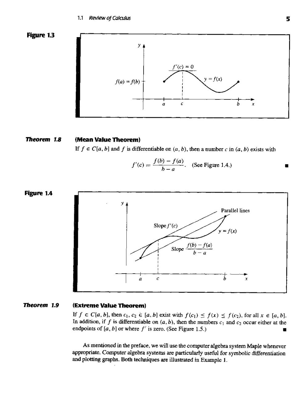
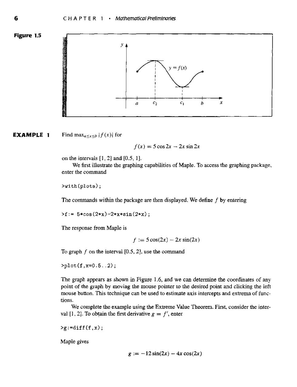
1.1 Review of Calculus 5 Figure 1.3 f'(c=0 f(a)=f(b)- y=f(x) Theorem 1.8 (Mean Value Theorem) If fC[a,]and f is differentiable on (a,b),then a number c in (a,b)exists with fe)(()(Sce Figure 1.4.) b-a Figure 1.4 Parallel lines Slopef"(c) y=f(r) Stope 1()-f(a) b-a Theorem 1.9 (Extreme Value Theorem) If f Cla,b],then c,c2 [a,b]exist with f(c)s f(x)s f(c2).for all x e [a,b] In addition,if f is differentiable on (then th nbersc either at th endpoints of Figure 1.5.) ■ As mentioned in the preface.we will use the mputer algebra system Maple whenever Compute
6 C HA PT E R 1.Mathematical Preliminaries Figure 1.5 EXAMPLE 1 Find maxasssb!f(x)for f(x)=5cos 2x-2x sin 2x on the intervais [1,2]and [0.5,1]. We first illu ate the graphing capabilities of Maple.To access the graphing package enter the command >with(plots); The commands within the package are then displayed.We define f by entering >f:=5*c0s(2*x)-2*x*81n(2*x); The response from Maple is f :=5 cos(2x)-2x sin(2x) To graph f on the interval [0.5,21.use the command >p1ot(f,x=0.5.2): The graph appears as shown in Figure 1.6,and we can determine the coordinates of any point of theg raph by moving the mouse pointer to the desired point and clicking the ieft buon This tchique a bedoinsand emoun using the Extreme Value Theorem.First,consider the inter Yal .2).Tootain the frst derivativeen >g:=diff(f,x); Maple gives 8 :=-12sin(2x)-4x cos(2x)
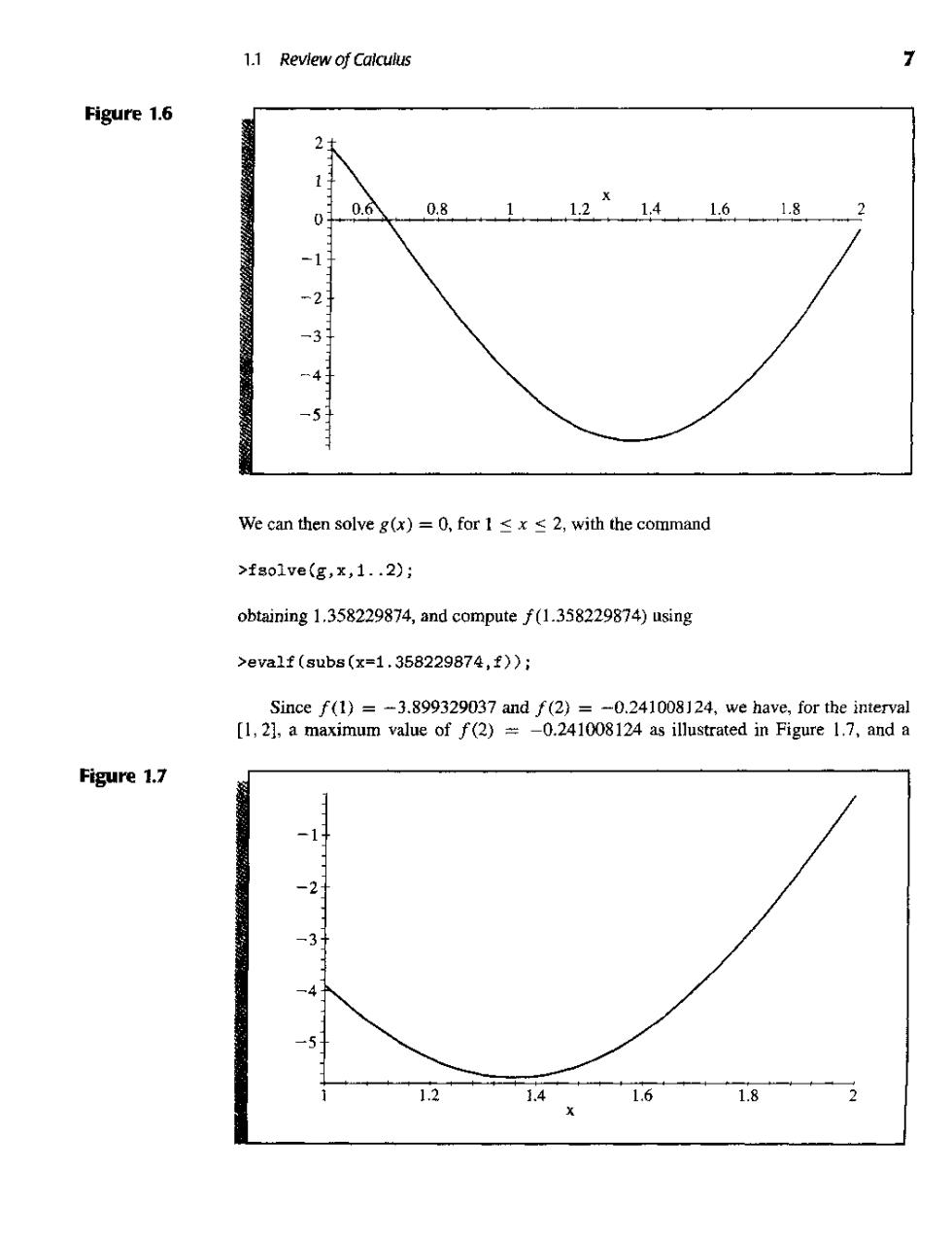
1.1 Review of Calculus Figure 1.6 2 1 0 0.81 1.21.41.6.1.8.2 -1 -2 -31 4 -5 We can then solve g(x)=0,for1≤x≤2,with the command >f8o1ve(g,x,1.2); obtaining 1.358229874,and compute f(1.358229874)using >eva1f(subs(x=1,358229874,f); Since f(1)=-3.899329037 and f(2)=-0.241008]24,we have,for the interval [1,2],a maximum value of f(2)=-0.241008124 as illustrated in Figure 1.7,and a Figure 1.7 -2 -3 1.2 1.4 1.6 1.8

minimum of approximately f(1.358229874)=-5.675301338.Hence, 5c0os2x-2 xsin2x1≈f1.3582298741=5.675301338. If we try to solve g(x)=0,for 0.5sx<1,we find that when we enter >fso1ve(g,x,0.5.1): Maple responds with fsolve(-12 sin(2x)-4a cos(2),x,.5.I) ion in this interval,and the maximum occurs at an endpoint.Hence f'is never 0 in [0.5,1].as shown in Figure 1.8.and,since f(0.5)=1.860040545 and f(1)=-3.899329037,we have 0,15c0s2x-2xsim2x=1f01=3.89329037. Figure 1.8 6 0.7 0.8 0.9 0 -2 -3 The other basic concept of calculus that will be used extensively is the Riemann inte- gral. Definition 1.10 The Riemann integral of the function f on the interval [a,]is the following limit,pro- vided it exists: ”fdx=n2f)△