Contents Iterative Techniques in Matrix Algebra 417 7.1 Norms of Vectors and Matrices 418 Eigenvalues and Eigenvectors 430 73 Iterative Techniques for Solving Linear Systems 437 7.4 Error Bounds and Iterative refinement 454 The Conjugate Gradient Mcthod 46s 7.6 Survey of Methods and Software 481 8 Approximation Theory 483 8.1 Discrete Least Squares Approximation 484 8.2 Orthogonal Polynomials and Least Squares Approximation 498 8.3 Chebyshev Polynomials and Economization of Power Series 507 8.4 Rational Function Approximation 517 8.5 Trigonometric Polynomial Approximation 529 8.6 Fast Fourier Transforms 537 8.7 Survey of Methods and Software 548 9 Approximating Eigenvalues 550 9.1 Linear Algebra and Eigenvalues 55t 9 The Po wer Method 560 Housebolder's Method 577 9.4 The QR Algorithm 585 9.5 Survey of Methods and Software 597 10 Numerical Solutions of Nonlinear Systems of Equations 600 10.1 Fixed Poimts for Functions of Several Variables 602 10.2 Newton's Method 611 10.3 Quasi-Newton Methods 620 10.4 Steepest Descent Techniques 628 10.5 Homotopy and Continuation Methods 635 10.6 Survey of Methods and Software 643

viii Contents 7 Boundary-Value Problems for Ordinary Differential Equations 645 11.1 The Linear Shooting Method 646 11.2 The Shooting Method for Nonlinear Problems 653 1.3 Finite-Difference Methods for Linear Problems 660 11.4 Fimite-Difference Methods for Nonlinear Problems 667 115 The Ravleigh-Ritz Method 672 11.6 Survey of Methods and Software 688 2 Numerical Solutions to Partial Differential Equations 691 12.t Elliptic Partial Differential Equations 694 12.2 Parabolic Partial Differential equations 704 12.3 Hyperbolic Partial Differential Equations 718 12.4 An Introduction to the Finite-Element Method 726 12.5 Survey of Methods and Software 741 Bibliography 743 Answers to Selected Exercises 753 Index 831

CHAPTER Mathematical Preliminaries Nbegnn chemistrycouesee the idel a PV=NRT, which relates the pressure P,volume V,temperature T,and number of moles N of.In this equation,R is a constant that depends on the measurement system. Suppose two experiments are conducted to test this law,using the same gas in each case.In the first experiment, P÷1.00atm, V=0.100m3, N=0.00420mol, R=0.08206. The ideal gas law predicts the temperature of the gas to be T=微-008=2015K-1rC (1.00)0.100) When we measure the temperature of the gas,we find that the true tem perature is 15C

CHA PTE R 1.Mathematical Preliminaries We then repeat the experiment using the same values of R and N, but increase the pressure by a factor of two and reduce the volume by the same factor.Since the product PV remains the same,the predicted temperature is still 17C,but we find that the actual temperature of the gas is now 19C. Clearly,the ideal gas law is suspect,but before concluding that the law is invalid in this situation,we should examine the data to see whether the error can be attributed to the experimental results.If so,we might be able to determine how much more accurate our experimental results would need to be to ensure that an error of this magnitude could not occur. m numerical analysis and is introduced in Section 1.2.This particular application is considered in Exercise 28 of that section. This chapter contains a short review of those topics from elementary single-variable calulus that will be needed in later chapters,togetber withan introduction to convergence,o analysis,and the machine representation of nunbers. 1.1 Review of Calculus The concepts of limir and of a function are fundamental to the study of calculus Definition 1.1 A function f defined on a set X of real numbers has the limit L at xo,written lim f(x)=L, if.given any real number>0,there exists a real number>0such that f()-LI<, whenever xX and 0<Ix-xol 8.(See Figure 1.1.) ■ Definition 1.2 Let f be a function defined on a set X of real numbers and xoeX.Then f is continuous at xoi证 lin f(x)=f(xo). The function f is continuons on the set if it is continuous at each number in X. ◆
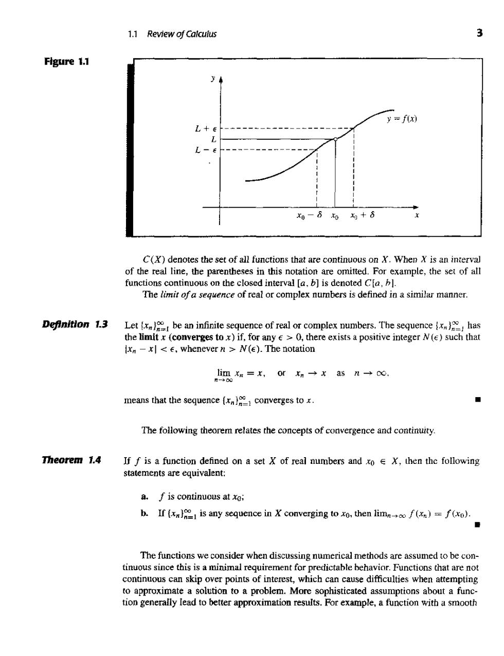
1.1 Review of Calculus Figure 1.1 JA y=f(x) L+∈ L-e 为-6名+6 C(X)denotes the set of all functions that are continuous on X.When X is an interval of thereal line,the parentheses in thisn ationare omitted.For xampe,the se of al functions continuous on the closed interval [a.b]is denoted C[a.b. The limit ofa sequence of real or complex numbers is defined in a similar manner. Definition 1.3 Let be an infinite sequence of real or complex numbers.The sedue erges tox)i ixm=K,0rn→xasn→心. means that the sequence (r converges to x. ■ The following theorem relates the concepts of convergence and continuity. Theorem 1.4 If f is a function defined on a set X of real numbers and xo X,then thc following statements are equivalent: a.f is continuous at xo: b.If (xloo is any sequence in X converging to xo,then limnof(n)=f(xo). The functions we consider when discussing numerical methods are assumed obe con- tinuous since this is a minimal requirement for predictable behavior.Functions that are not continuous can skip over points of interest,which can cause difficulties when attempting to approximate a solution to a problem.More sophisticated assumptions about a func- tion generally lead to better approximation results.For example,a function with a smooth