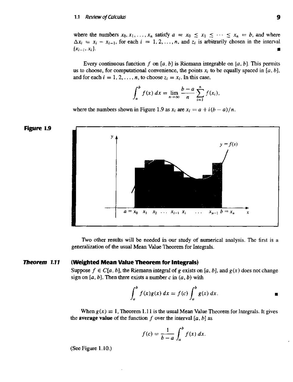
1.1 Review of Calculus 9 where the numberso,satisfy a=0≤≤≤xn=b,and where Axi =xi-xi-1,for each i=1,2,.,n,and zi is arbitrarily chosen in the interval {x-1,x 直 Every continuous function f on [a.b]is Riemann integrable on a,].This permit and for eachi=1.2,.n,to choose=x.In this case. where the numbers shown in Figure 1.9 as xi arexi=a+i(b-a)/n. Figure 1.9 y=f(x) 为为.-1 xn-1b= Two other results will be needed in our study of numerical analysis.The first is a generalization of the usual Mean Value Theorem for Integrals. Theorem 1.11 (Weighted Mean Value Theorem for Integrals) Suppose fCfa,bl,the Riemann integral of g exists on [a.b],and g(x)does not change sign on Then there existsanum)wth When g(x)=1,Theorem 1.11 is the usual Mean Value Theorem for Integrals.It gives the average value of the function f over the interval [a,b as 1 f(e)=bal f()dz. (See Figure 1.10.)
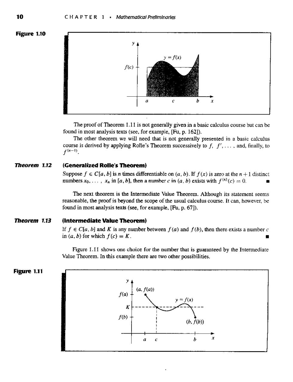
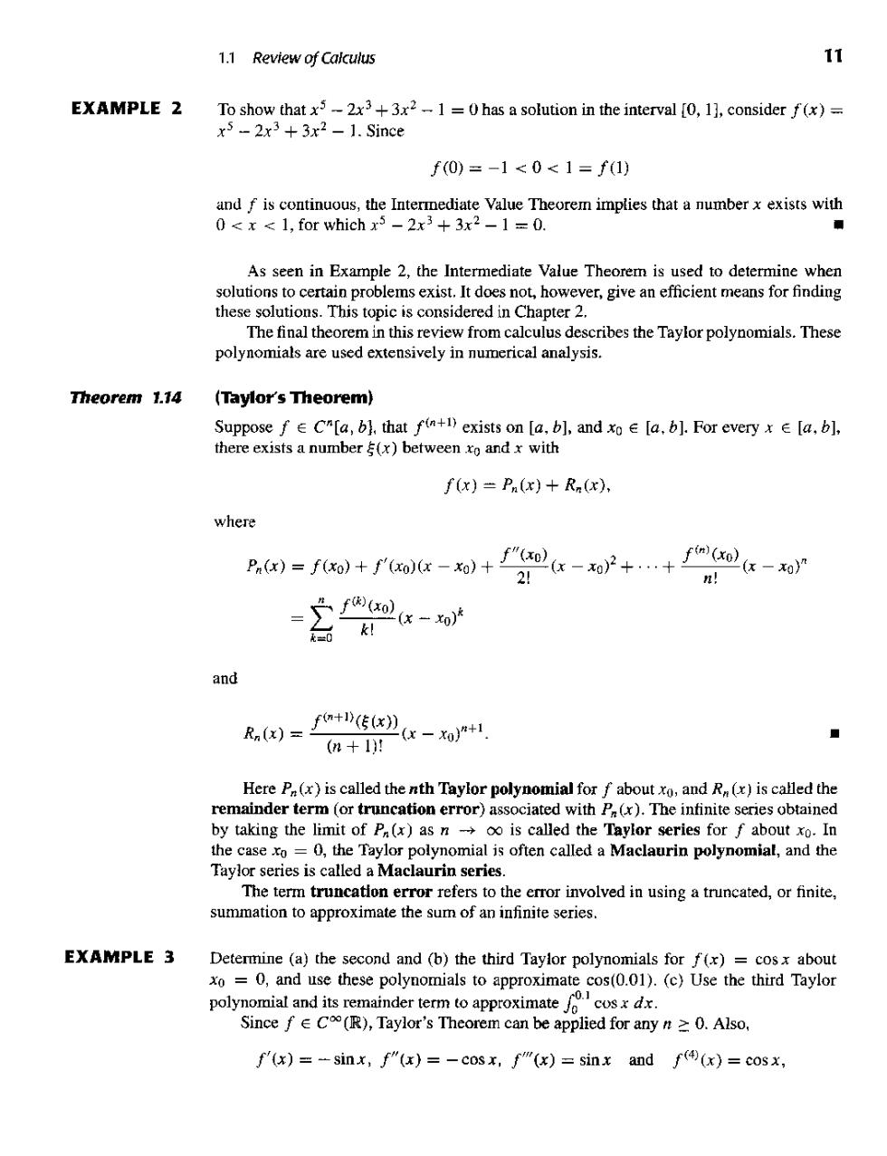
10 Figure 1.10 y=f(x) c b The proof of Theorem 1.11 is not generally given in a basic calculus course but can be found in most analysis texts(see,for example,[Fu,p.1621). The other theorem we will need that is not generally presented in a basic calculus course is derived by applying Rolle's Theorem successively to f,f,.and,finally,to f-). Theorem 1.12 (Generalized Rolle's Theorem) Suppose fCla,b]isn times differentiable on(a,b).If f(x)is zero at then+1 distinct numbers xo.,xm in [a,b],then a number c in (a,b)exists with f(n)(c)=0. The next theorem is the Intermediate Value Theorem.Although its statement seems reasonable,the proof is beyond the scope of the usual calculus course.It can,however,be found in most analysis texts (see,for example,[Fu,p.67)). Theorem 1.13 (Intermediate Value Theorem) If f e Cla,bj and K is any number between f(a)and f(b),then there exists a number c in (a,b)for which f(c)=K. ■ Figure 1.1I shows one choice for the number that is guaranteed by the Intermediate Value Theorem.In this example there are two other possibilities. Figure 1.11 y (a.f(a)) f(a) =f(x f(b)-
1.1 Review of Calculus 11 EXAMPLE 2 To show that x5-2x3+3x2-1 =0 has a solution in the interval [0,1],consider f(x)= x5-2x3+3x2-1.Since f(0)=-1<0<1=f(1) and f is continuous,the Intermediate Value Theorem implies that a numberx exists with 0<x<1.for whichx-2x+3x-1=0. when soloionstocertaio.problem s exis these solutions This topic is considered in Chapter 2. The final theorem in this review from calculus describes the Taylor polynomials.These polynomials are used extensively in numerical analysis. Theorem 1.14 (Taylor's Theorem) f(x)=P(x)+R(x). where a)=fo+fo-0+u-o产++fa@g-0 2 n! =乃fox-o and (+1)! Here P(x)is called the nth Taylor polynomial for f about xo,and R(x)is called the remainder term (or truncation error) ciated with P (x).The infinite eries obtained by taking thein t of Pa(x)as n- is called theT series abou In the case o- or polynomial is often called a Maclaurin polynomial,and the Tay iscaleda The term truncation error refers to the error involved in using a truncated,or finite, summation to approximate the sum of an infinite series. EXAMPLE 3 Determine (a)the second and (b)the third Taylor polynomials forf(x)=cosx about xo=0,and use these polynomials to approximate cos(0.01).(c)Use the third Taylor polynomial and its remainder term to approximatecosx dx. Since f C(R),Taylor's Theorem can be applied for any n0.Also, f'(x)=-sinx,f"(x)=-cosx,f"M(x)=sinx and f((x)=cosx
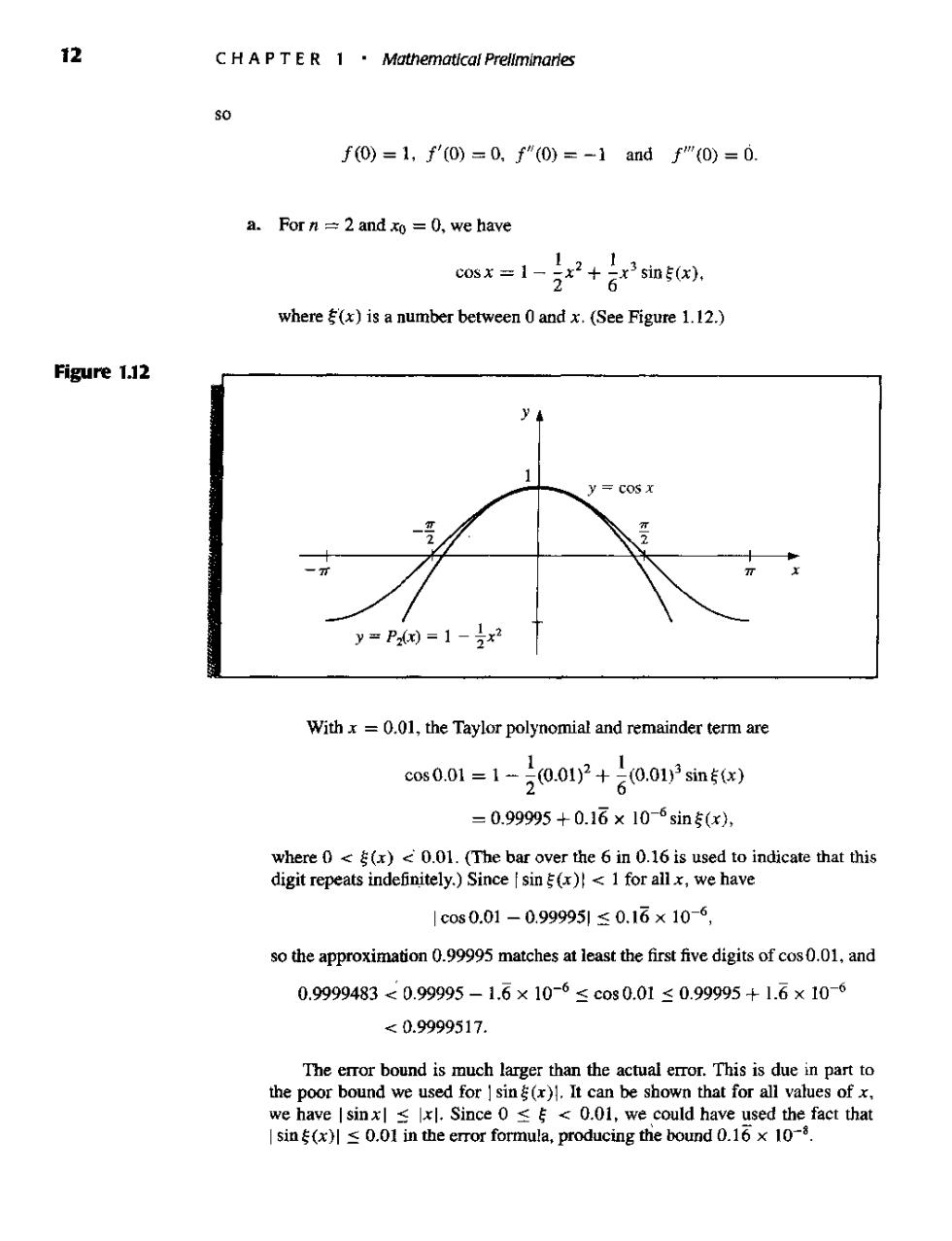
12 C HA PT E R 1.Mathematical Prellminarles % f0=1,f'0)=0,f"0)=-】andf"0)=0. a.For n =2 and xo=0,we have cosx=1-2x2+石2sin56. where(x)is a number between 0 and x.(See Figure 1.12.) Figure 1.12 y y=P2=1-x2 Withx=0.01,the Taylor polynomial and remainder term are cos01=1-0oP+0013sm5t) =0.99995+0.16×10⁶sin5x), where().01.(The bar over the 6 in 0.16 is used to indicate that this digit repeats indefinitely.)Since sin(!1for allx,we have 1c0s0.01-0.999951≤0.16x10⁻⁶, so the approximation 0.99995 matches at least the first five digits of cos0.01,and 0.9999483<0.99995-1.6×10⁶≤cos0.01≤0.99995+1.6×10⁶ <0.9999517. The error bound is much larger than the actual error.This is due in part to the poor bound we used for I sin()1.It can be shown that for all values ofx. we have I sinxs xl.Since 0 0.01,we could have used the fact that Isin(x)<0.01 in the error formula,producing the bound 0.16 x 10⁻⁸
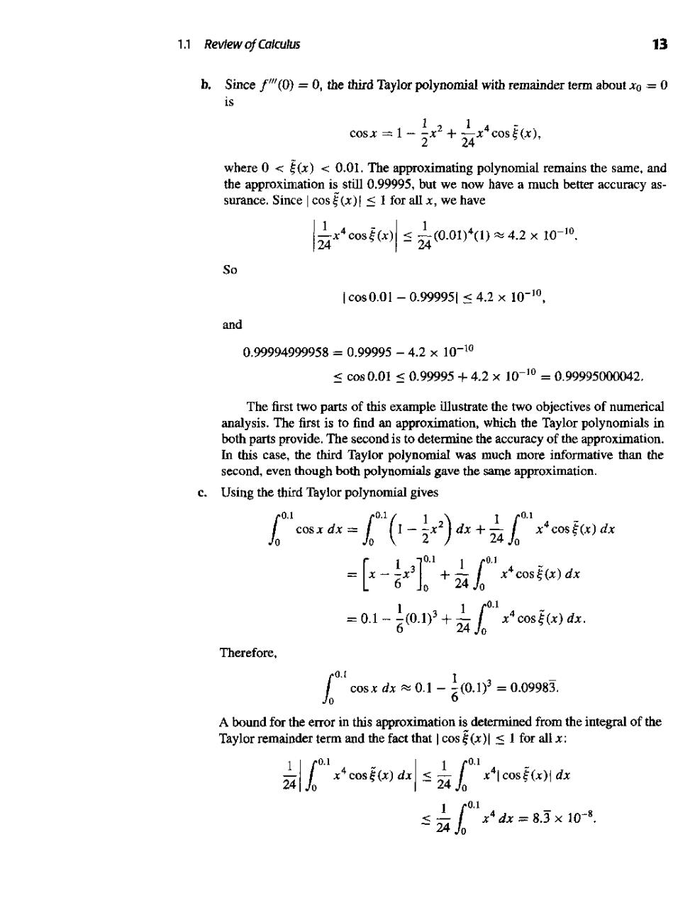
1.1 Revlew of Calculus 13 b.Since f(0)=0,the third Taylor polynomial with remainder term about xo=0 is co() where 0)<0.01.The approximating polynomial remains the same,and the approximation is still 0.99995,but we now have a much better accuracy as- surance.Since cos()!s I for all x,we have 2acos56x≤240.01≈42×100 So 1cos0.01-0.999951≤4.2×10⁻¹⁰ and 0.99994999958=0.99995-4.2×10¹⁰ ≤c0s0.01≤0.99995+4.2×10-10=0.99995000042. The first two parts of this example illustrate the two objectives of numerical analysis.The first is to find an approximation,which the Taylor polynomials in both parts provide.The second is to determine the accuracy of the approximation. In this case,the third Taylor polynomial was much more informative than the second,even though both polynomials gave the same approximation. c.Using the third Taylor polynomial gives 01 xcos(x)dx =01-言0+co5 Therefore. “cos≈0.1-。0.1y=0.09983 A bound for the error in this approximation is determined from the integral of the Taylor remainder term and the fact that cos(x)s I for all x: 10. ≤240 x4d=8.3×10⁸