9.6.SUMMARY OF THE IMC DESIGN PROCEDURE 199 9.6 Summary of the IMC Design Procedure The required information for the IMC design is the same as that for stable sys- tems:process model,input type.performance specifications and uncertainty in- formation.The input specification requires some care.If the physical disturbance enters at the plant input,the disturbance used in the design procedure has to include the unstable system poles for the resulting controller to yield offset free performance. Design Procedure Step 1:Nominal Performance The stabilizing H2-optimal controller g is determined which minimizes (1-p^g)v2 for the specifed input u".The optimal controller g can be found explicitly from 9.2-4). 9H=pbr)1{(:6pA}16i}. (9.2-4) If all the unstable plant/disturbance poles are at the origin.the entries in Table 8.1-1 can be used to find qi for typical inputs. The controller g is then modified as described in Sec.9.2-2 to eliminate the problems of intersample rippling: G=GHq-B 9.2-20) Step 2:Robust Stability and Robust Perjormance The controller g is augmented by the IMC filter f q=af In order for q to be stabilizing f has to be unity at all unstable system p"and input v'poles 1,...,T.When the poles outside the UC are distinct,the one- parameter fiiter is determined through Thm.9.3-1.The filter poles are a subset of the closed-loop poles.If they are made much slower than the mirror images of the poles of p"outside the UC undesirable performance and robustness properties result. Robust Stability.Increase a (or A in a =e-T/A)until gfm|<1,0≤w≤x/T 9.4-2) is satisfied for a≥a
200 CHAPTER 9.SISO DESIGN FOR UNSTABLE SAMPLED-DATA SYSTEMS Robust Performance.Increase a,starting from a',until the following condition is met 19Ea+1-p9w≤1,0≤≤/T (8.4-1) where a(s)=a(eT)f(esT)ho(s)(s)/T (7.5-10) 9.7 Application:Distillation Column Base Level Control This example was discussed in detail in Sec.5.7.1.It is briefly considered here again,because some interesting issues arise when a digital controller is designed for the process. The process model is (s)=(1-2es) (5.7-1) Let us select a sampling time T=0/N,where N is an integer.Then the zero- order hoid discrete equivalent is e)=2Css明=1-2z-{as}=任-2 9.7-1) In this very special case we find that if is a finite zero of p(s),then eT is a zero of p"()and therefore is a zero of p"(esT).This mapping does not hold for zeros in general,although it is always true for the poles of p(s)and p(). Because of this mapping the zeros of p()that appear as poles of gu(=)are cancelled by zeros of p(s)in (7.5-6).Therefore,any such zeros close to (-1.0) do not produce intersample rippling even if the modifcation described in Sec. 9.2.2 is not made.However,this does not mean that the behavior of the coatrol system will deteriorate if the suggested modification is introduced.Indeed,the steps proposed in Sec.9.2 will result in a weil-performing controller,regardless of whether()suffers from rippling problems or not. Let us proceed to illustrate this point by simulating the response for the two controllers for a ramp disturbance d(s)=s-2.For the simulations we choose 0=5 and T=1,which implies that N=5.It follows from (9.7-1)that the zeros of p"(z)are located at 21/5ek/5,=0.1,2,3,4,where 21/5 indicates the real fifth root of 2.Two of these zeros(the ones that correspond to k=2,3)have
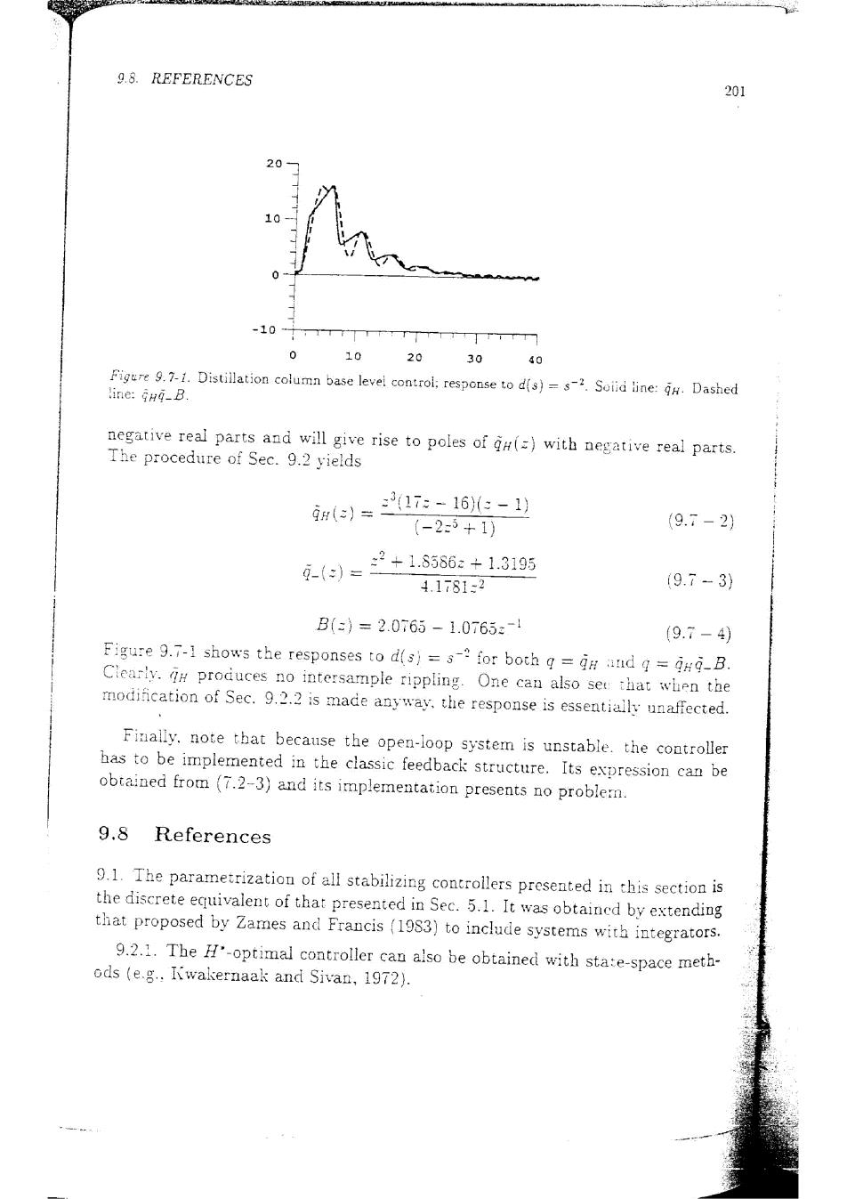
9.8.REFERENCES 201 20 10 0 -10 0 10 20 30 40 Figure 9.7-1.Distillation column base level control:response to d(s)=s-2.Soiid line:GH.Dashed line:Gng_B. negative real parts and will give rise to poles of gH(=)with negative real parts. The procedure of Sec.9.2 yields H()= 17:-16e-1) (-2-5+1) (9.7-2) 9-()= 2+1.8586:+1.3195 4.1781-2 19.7-3) B(-)=2.0765-1.0765:-1 (9.7-4) Figure 9.7-1 shows the responses to d(s)=s-for both q=di and q=jng-B. Clearly.produces no intersample rippling.One can also see that when the modification of Sec.9.2.2 is made anyway.the response is essentially unaffected. Finally.note that because the open-loop system is unstable.the controller has to be implemented in the classic feedback structure.Its expression can be obtained from (7.2-3)and its implementation presents no problem. 9.8 References 9.1.The parametrization of all stabilizing controllers presented in this section is the discrete equivalent of that presented in Sec.5.1.It was obtained by extending that proposed by Zames and Francis (1983)to include systems with integrators. 9.2.1.The H-optimal controller can also be obtained with sta:e-space meth- ods (e.g.,I(wakernaak and Sivan,1972)
Part III CONTINUOUS MULTL-INPUT MULTI-OUTPUT SYSTEMS
Chapter 10 FUNDAMENTALS OF MIMO FEEDBACK CONTROL In the first section of this chapter some concepts from linear system theory are summarized.The singular value decomposition,which plays a key role in the rest of the book,is covered in detail.The control problem formulation introduced for SISO systems (model uncertainty description,input definition.performance objectives)is generalized to multivariable systems.The Nyquist stability criterion is extended to handle MIMO systems. 10.1 Definitions and Basic Principles This introductory section is a self-contained summary.For the proofs and a deeper understanding the reader is referred to a basic text on linear systems. 10.1.1 Modeling In te time domain a linear time.invariant finite dimensional system can be described by the syster of differential and algebraic equations- 主=Ax+Bu (10.1-1) y三Cx+Du (10.1-2) where r∈Rry∈R”and u e_R"are the state,output and input vectors respectively and A,B,C,and D are constant matrices of apprepriate dimensions. Taking the Laplace transform of (10.1-1)and (10.1-2)with zero initial conditions sIx(s)=Ax(s)+Bu(s) (10.1-3) or x(s)=(sI-A)Bu(s) (10.1-4) y(s)=Ca(s)+Du(s) (10.1-5) 205