Chapter 2 Classical Analysis Methods 4口,+@,4定4=定0C Zhang.W.D..CRC Press.2011 Version 1.0 1/64
Chapter 2 Classical Analysis Methods Zhang, W.D., CRC Press, 2011 Version 1.0 1/64
Classical Analysis Methods 12.1 Process Dynamic Responses 2 2.2 Rational Approximations for Time Delay 3 2.3 Time Domain Performance Indices 42.4 Frequency Response Analysis 52.5 Transformation of Two Commonly Used Models 62.6 Design Requirements and Method Comparison 4口,4@,4定4定0C Zhang.W.D..CRC Press.2011 Version 1.0 2/64
Classical Analysis Methods 1 2.1 Process Dynamic Responses 2 2.2 Rational Approximations for Time Delay 3 2.3 Time Domain Performance Indices 4 2.4 Frequency Response Analysis 5 2.5 Transformation of Two Commonly Used Models 6 2.6 Design Requirements and Method Comparison Zhang, W.D., CRC Press, 2011 Version 1.0 2/64
Section 2.1 Process Dynamic Responses 2.1 Process Dynamic Responses Plant Description Different plants may be described by the same model: Distillation column,paper-making machine,disk,maglev, Description:Linear time-invariant causal model G(t),where t is the continuous time variable.G(s)denote its transfer function. Causality:G(t)=0 for t<0.Implication:the output depends only on the current and the previous inputs Properness: Proper-G(s)ls=joo is finite(the degree of denominator is greater than or equals the degree of numerator) ② Strictly proper-G(s)ls=j=0(the degree of denominator is greater than the degree of numerator) ③ Bi-proper-G(s)ls=jo is a nonzero constant(the degree of denominator equals the degree of numerator) ④Improper--Not proper 定9QC Zhang.W.D..CRC Press.2011 Version 1.0 3/64
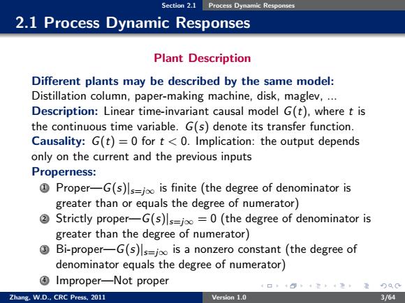
Section 2.1 Process Dynamic Responses 2.1 Process Dynamic Responses Plant Description Different plants may be described by the same model: Distillation column, paper-making machine, disk, maglev, ... Description: Linear time-invariant causal model G(t), where t is the continuous time variable. G(s) denote its transfer function. Causality: G(t) = 0 for t < 0. Implication: the output depends only on the current and the previous inputs Properness: 1 Proper—G(s)|s=j∞ is finite (the degree of denominator is greater than or equals the degree of numerator) 2 Strictly proper—G(s)|s=j∞ = 0 (the degree of denominator is greater than the degree of numerator) 3 Bi-proper—G(s)|s=j∞ is a nonzero constant (the degree of denominator equals the degree of numerator) 4 Improper—Not proper Zhang, W.D., CRC Press, 2011 Version 1.0 3/64
Section 2.1 Process Dynamic Responses Stable Plants with Time Delays When the original mass or energy equilibrium is upset by a change at the input,the output will eventually reach a new equilibrium. Feature:Do not have closed RHP poles 2.0 1.3 1.0 0.5 0.0 Time 4口+0:4定4生定9QC Zhang.W.D..CRC Press.2011 Version 1.0 4/64
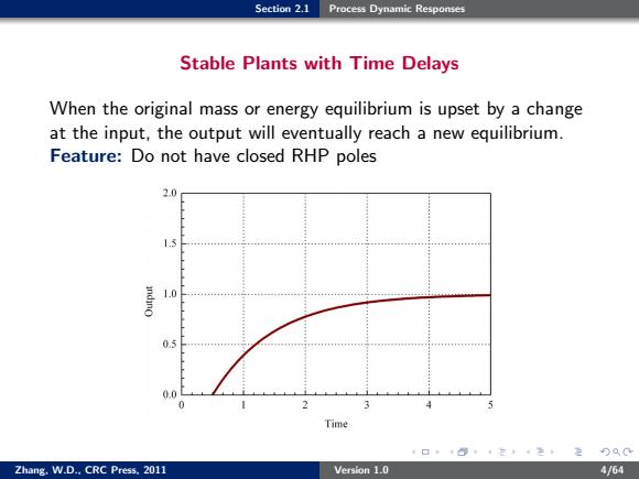
Section 2.1 Process Dynamic Responses Stable Plants with Time Delays When the original mass or energy equilibrium is upset by a change at the input, the output will eventually reach a new equilibrium. Feature: Do not have closed RHP poles Zhang, W.D., CRC Press, 2011 Version 1.0 4/64

Section 2.1 Process Dynamic Responses Models of Stable Plants K 6=n9+2s+.m5+de: K-Real constant denoting the static gain 0-Positive real constant denoting the time delay Ti(i =1,2,...n)-Have positive real parts and denote time constants The first-order model frequently used in practice: G(s)= e-s rs+1 The model can well be illustrated by utilizing a shower 4口,+@,4定4=定0C Zhang.W.D..CRC Press.2011 Version 1.0 5/64
Section 2.1 Process Dynamic Responses Models of Stable Plants G(s) = K (τ1s + 1)(τ2s + 1)...(τns + 1) e −θs K—Real constant denoting the static gain θ—Positive real constant denoting the time delay τi(i = 1, 2, ..., n)—Have positive real parts and denote time constants The first-order model frequently used in practice: G(s) = K τ s + 1 e −θs The model can well be illustrated by utilizing a shower Zhang, W.D., CRC Press, 2011 Version 1.0 5/64