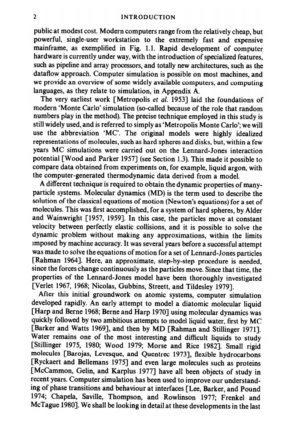
2 INTRODUCTION public at modest cost.Modern computers range from the relatively cheap,but powerful,single-user workstation to the extremely fast and expensive mainframe,as exemplified in Fig.1.1.Rapid development of computer hardware is currently under way,with the introduction of specialized features, such as pipeline and array processors,and totally new architectures,such as the dataflow approach.Computer simulation is possible on most machines,and we provide an overview of some widely available computers,and computing languages,as they relate to simulation,in Appendix A. The very earliest work [Metropolis et al.1953]laid the foundations of modern 'Monte Carlo'simulation (so-called because of the role that random numbers play in the method).The precise technique employed in this study is still widely used,and is referred to simply as'Metropolis Monte Carlo';we will use the abbreviation 'MC.The original models were highly idealized representations of molecules,such as hard spheres and disks,but,within a few years MC simulations were carried out on the Lennard-Jones interaction potential [Wood and Parker 1957](see Section 1.3).This made it possible to compare data obtained from experiments on,for example,liquid argon,with the computer-generated thermodynamic data derived from a model. A different technique is required to obtain the dynamic properties of many- particle systems.Molecular dynamics(MD)is the term used to describe the solution of the classical equations of motion (Newton's equations)for a set of molecules.This was first accomplished,for a system of hard spheres,by Alder and Wainwright [1957,1959].In this case,the particles move at constant velocity between perfectly elastic collisions,and it is possible to solve the dynamic problem without making any approximations,within the limits Imposed by machine accuracy.It was several years before a successful attempt was made to solve the equations of motion for a set of Lennard-Jones particles [Rahman 1964].Here,an approximate,step-by-step procedure is needed, since the forces change continuously as the particles move.Since that time,the properties of the Lennard-Jones model have been thoroughly investigated [Verlet 1967,1968;Nicolas,Gubbins,Streett,and Tildesley 1979]. After this initial groundwork on atomic systems,computer simulation developed rapidly.An early attempt to model a diatomic molecular liquid [Harp and Berne 1968;Berne and Harp 1970]using molecular dynamics was quickly followed by two ambitious attempts to model liquid water,first by MC [Barker and Watts 1969],and then by MD [Rahman and Stillinger 1971]. Water remains one of the most interesting and difficult liquids to study [Stillinger 1975,1980;Wood 1979;Morse and Rice 1982].Small rigid molecules [Barojas,Levesque,and Quentrec 1973],flexible hydrocarbons [Ryckaert and Bellemans 1975]and even large molecules such as proteins [McCammon,Gelin,and Karplus 1977]have all been objects of study in recent years.Computer simulation has been used to improve our understand- ing of phase transitions and behaviour at interfaces [Lee,Barker,and Pound 1974;Chapela,Saville,Thompson,and Rowlinson 1977;Frenkel and McTague 1980].We shall be looking in detail at these developments in the last
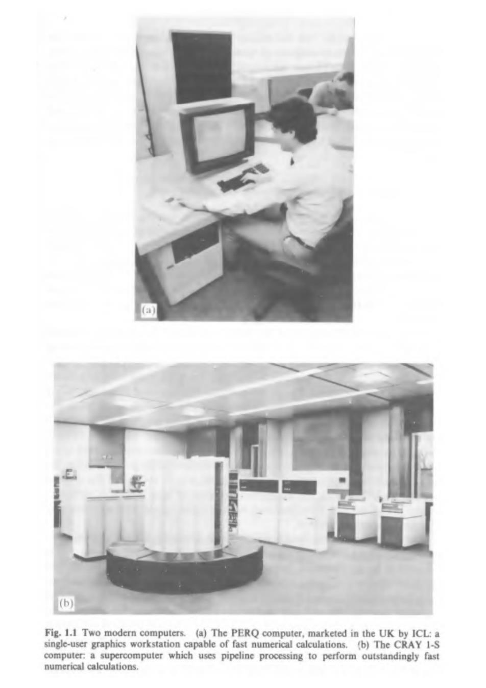
a (b) Fig.1.1 Two modern computers.(a)The PERQ computer,marketed in the UK by ICL:a single-user graphics workstation capable of fast numerical calculations.(b)The CRAY 1-S computer:a supercomputer which uses pipeline processing to perform outstandingly fast numerical calculations
INTRODUCTION chapter of this book.The techniques of computer simulation have also advanced,with the introduction of'non-equilibrium'methods of measuring transport coefficients [Lees and Edwards 1972;Hoover and Ashurst 1975; Ciccotti,Jacucci,and McDonald 1979],the development of 'stochastic dynamics'methods [Turq,Lantelme,and Friedman 1977],and the incorpor- ation of quantum mechanical effects [Corbin and Singer 1982;Ceperley and Kalos 1986].Again,these will be dealt with in the later chapters.First,we turn to the questions:What is computer simulation?How does it work?What can it tell us? 1.2 Computer simulation:motivation and applications Some problems in statistical mechanics are exactly soluble.By this,we mean that a complete specification of the microscopic properties of a system(such as the Hamiltonian of an idealized model like the perfect gas or the Einstein crystal)leads directly,and perhaps easily,to a set of interesting results or macroscopic properties(such as an equation of state like PV=NkeT).There are only a handful of non-trivial,exactly soluble problems in statistical mechanics [Baxter 1982];the two-dimensional Ising model is a famous example. Some problems in statistical mechanics,while not being exactly soluble, succumb readily to analysis based on a straightforward approximation scheme.Computers may have an incidental,calculational,part to play in such work,for example in the evaluation of cluster integrals in the virial expansion for dilute,imperfect gases.The problem is that,like the virial expansion,many 'straightforward'approximation schemes simply do not work when applied to liquids.For some liquid properties,it may not even be clear how to begin constructing an approximate theory in a reasonable way.The more difficult and interesting the problem,the more desirable it becomes to have exact results available,both to test existing approximation methods and to point the way towards new approaches.It is also important to be able to do this without necessarily introducing the additional question of how closely a particular model(which may be very idealized)mimics a real liquid,although this may also be a matter of interest.. Computer simulations have a valuable role to play in providing essentially exact results for problems in statistical mechanics which would otherwise only be soluble by approximate methods,or might be quite intractable.In this sense,computer simulation is a test of theories and,historically,simulations have indeed discriminated between well-founded approaches(such as integral equation theories [Hansen and McDonald 1986])and ideas that are plausible but,in the event,less successful (such as the old cell theories of liquids [Lennard-Jones and Devonshire 1939a,1939b]).The results of computer simulations may also be compared with those of real experiments.In the first place,this is a test of the underlying model used in a computer simulation
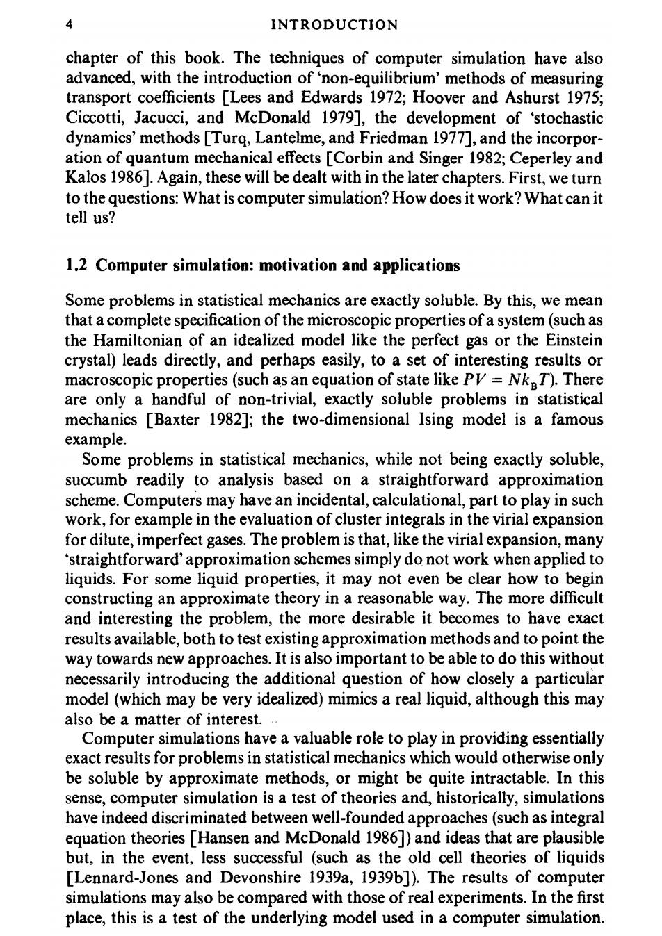
COMPUTER SIMULATION:MOTIVATION AND APPLICATIONS 5 Eventually,if the model is a good one,the simulator hopes to offer insights to the experimentalist,and assist in the interpretation of new results.This dual role of simulation,as a bridge between models and theoretical predictions on the one hand,and between models and experimental results on the other,is illustrated in Fig.1.2.Because of this connecting role,and the way in which simulations are conducted and analysed,these techniques are often termed computer experiments'. REAL MAKE MODEL LIQUIDS MODELS LIQUIDS PERFORM CARRY OUT CONSTRUCT EXPERIMENTS COMPUTER APPROXIMATE SIMULATIONS THEORIES EXPERIMENTAL EXACT RESULTS FOR THEORETICAL RESULTS MODEL PREDICTIONS, COMPARE COMPARE TESTS OF TESTS OF MODELS THEORIES Fig.1.2 The connection between experiment,theory,and computer simulation. Computer simulation provides a direct route from the microscopic details of a system (the masses of the atoms,the interactions between them,molecular geometry etc.)to macroscopic properties of experimental interest (the equation of state,transport coefficients,structural order parameters,and so on).As well as being of academic interest,this type of information is technologically useful.It may be difficult or impossible to carry out experiments under extremes of temperature and pressure,while a computer
6 INTRODUCTION simulation of the material in,say,a shock wave,a high-temperature plasma,a nuclear reactor,or a planetary core,would be perfectly feasible.Quite subtle details of molecular motion and structure,for example in heterogeneous catalysis,fast ion conduction,or enzyme action,are difficult to probe experimentally,but can be extracted readily from a computer simulation Finally,while the speed of molecular events is itself an experimental difficulty, it presents no hindrance to the simulator.A wide range of physical phenomena, from the molecular scale to the galactic [Hockney and Eastwood 1981],may be studied using some form of computer simulation. In most of this book,we will be concerned with the details of carrying out simulations(the central box in Fig.1.2).In the rest of this chapter,however,we deal with the general question of how to put information in(i.e.how to definea model of a liquid)while in Chapter 2 we examine how to get information out (using statistical mechanics). 1.3 Model systems and interaction potentials 1.3.1 Introduction In most of this book,the microscopic state of a system may be specified in terms of the positions and momenta of a constituent set of particles:the atoms and molecules.Within the Born-Oppenheimer approximation,it is possible to express the Hamiltonian of a system as a function of the nuclear variables,the (rapid)motion of the electrons having been averaged out.Making the additional approximation that a classical description is adequate,we may write the Hamiltonian of a system of N molecules as a sum of kinetic and potential energy functions of the set of coordinates qi and momenta p:of each molecule i.Adopting a condensed notation q=(91,92,,9N) (1.1a) P=(P1,P2,.·,PN (1.1b) we have 光(q,p)=(p)+(q). (1.2) The generalized coordinates q may simply be the set of Cartesian coordinates ri of each atom (or nucleus)in the system,but,as we shall see,it is sometimes useful to treat molecules as rigid bodies,in which case q will consist of the Cartesian coordinates of each molecular centre of mass together with a set of variables that specify molecular orientation.In any case,p stands for the appropriate set of conjugate momenta.Usually,the kinetic energy takes the form ∑p/2m (1.3) =1