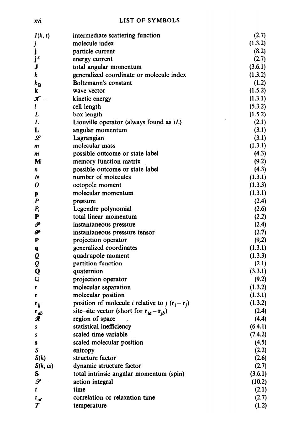
XVi LIST OF SYMBOLS I(k,t) intermediate scattering function (2.7) molecule index (1.3.2) j particle current (8.2) j energy current 2.7) J total angular momentum (3.6.1) k generalized coordinate or molecule index (1.3.2) k Boltzmann's constant (1.2) k wave vector (1.5.2) kinetic energy (1.3.1) cell length (5.3.2) L box length (1.5.2) L Liouville operator (always found as iL) (2.1) L angular momentum (3.1) 9 Lagrangian (3.1) m molccular mass (1.3.1) m possible outcome or state label (4.3) M memory function matrix (9.2) n possible outcome or state label (4.3) N number of molecules (1.3.1) 0 octopole moment (1.3.3) P molecular momentum (1.3.1) P pressure (2.4) P Legendre polynomial (2.6) P total linear momentum (2.2) e instantaneous pressure (2.4) P instantaneous pressure tensor (2.7) P projection operator (9.2) generalized coordinates (1.3.1) e quadrupole moment (1.3.3) o partition function (2.1) Q quaternion (3.3.1) Q projection operator (9.2) molecular separation (1.3.2) molecular position (1.3.1) r订 position of molecule i relative to j(ri) (1.3.2) Ia site-site vector (short for ria-jb) (2.4 凳 region of space (4.4) statistical inefficiency (6.4.1) scaled time variable (7.4.2) 3 scaled molecular position (4.5) S entropy (2.2) S(k) structure factor (2.6 Sk,ω) dynamic structure factor (2.7 S total intrinsic angular momentum (spin) (3.6.1) 9 action integral (10.2) t time (2.1) t correlation or relaxation time (2.7) T temperature (1.2)
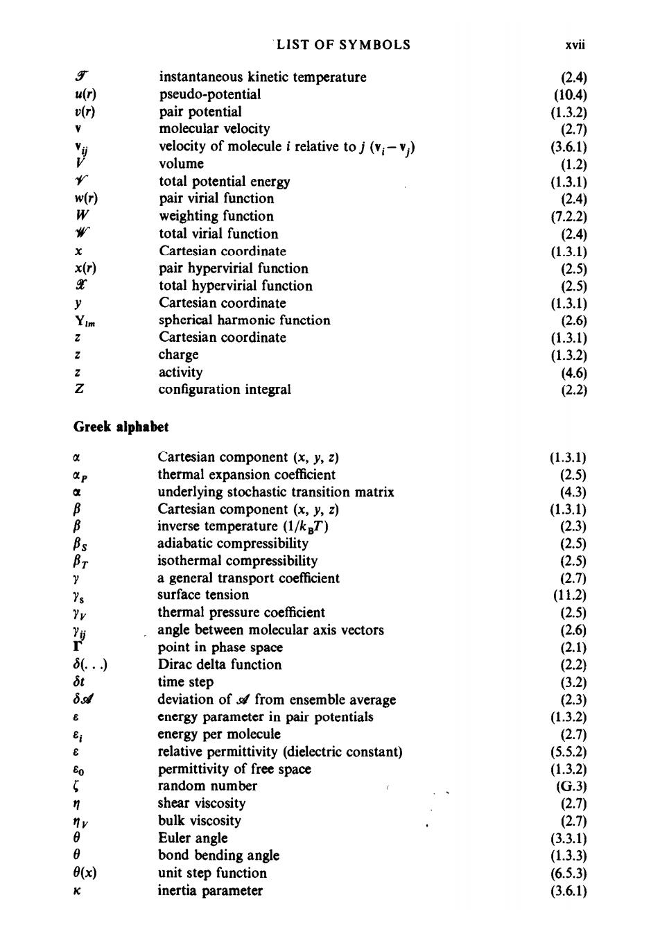
LIST OF SYMBOLS xvil $ instantaneous kinetic temperature 2.4) u(r) pseudo-potential (10.4) vr) pair potential (1.3.2) molecular velocity (2.7) velocity of molecule i relative to j (vi-vi) (3.6.1) V volume (1.2) r total potential energy (1.3.1) w(r) pair virial function 2.4) W weighting function (7.2.2) total virial function (2.4) Cartesian coordinate (1.3.1) x(r) pair hypervirial function (2.5 total hypervirial function (2.5) y Cartesian coordinate (1.3.1) im spherical harmonic function (2.6) Cartesian coordinate (1.3.1) charge (1.3.2) activity (4.6) i configuration integral (2.2) Greek alphabet 中 Cartesian component (x,y,z) (1.3.1) P thermal expansion coefficient (2.5) a underlying stochastic transition matrix (4.3) B Cartesian component (x,y,z) (1.3.1) B inverse temperature (1/kBT) (2.3) adiabatic compressibility (2.5) Br isothermal compressibility 2.5) y a general transport coefficient (2.7) Ys surface tension (11.2) Yv thermal pressure coefficient (2.5) Y angle between molecular axis vectors (2.6) point in phase space (2.1) 8(.) Dirac delta function (2.2) δt time step (3.2) 6ad deviation of/from ensemble average (2.3) energy parameter in pair potentials (1.3.2) Ei energy per molecule (2.7) e relative permittivity (dielectric constant) (5.5.2) Eo permittivity of free space (1.3.2) random number (G.3) 夕 shear viscosity (2.7 nv bulk viscosity (2.7) Euler angle (3.3.1) 8 bond bending angle (1.3.3) 0(x) unit step function (6.5.3) K inertia parameter (3.6.1)
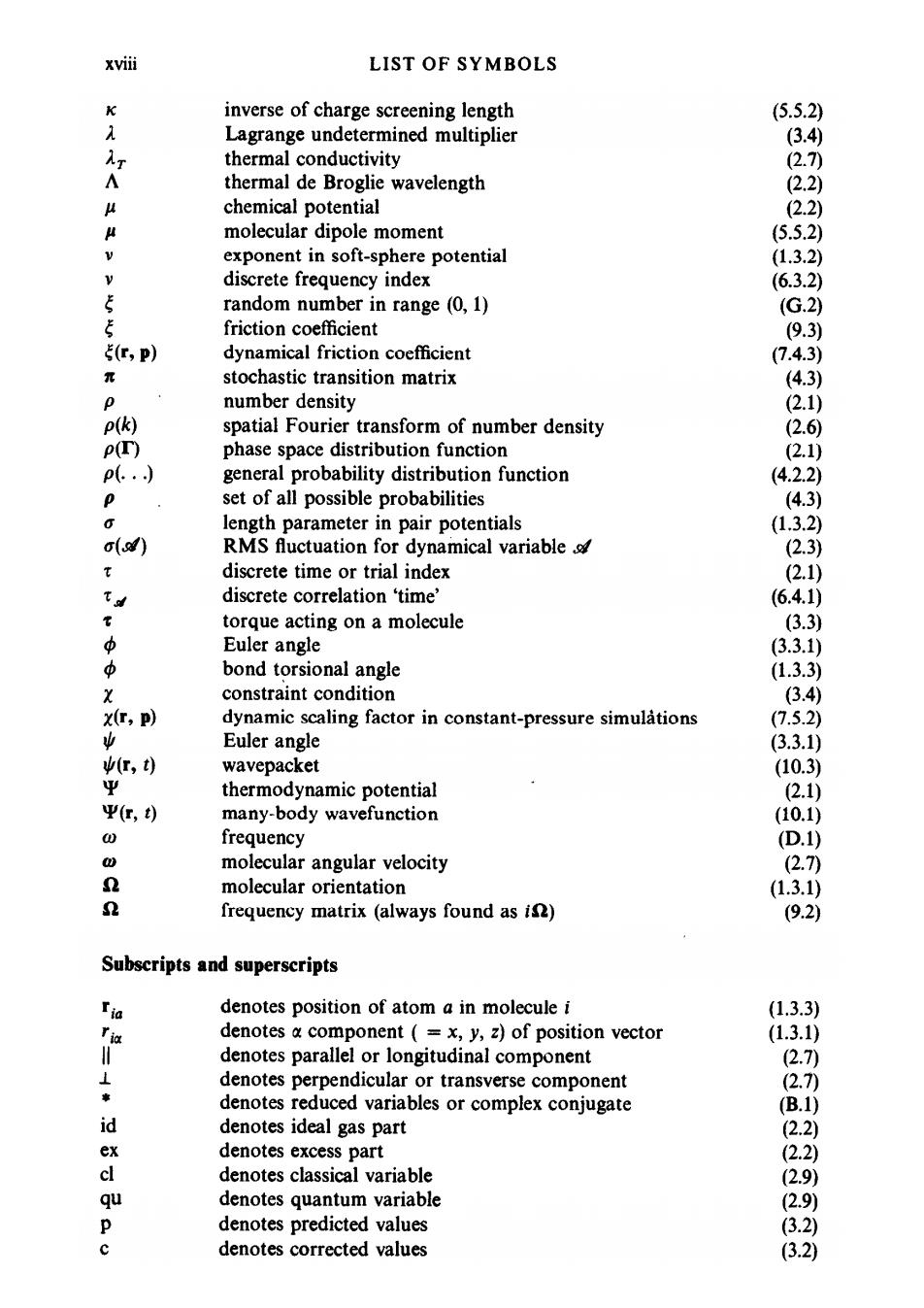
xviii LIST OF SYMBOLS 平 inverse of charge screening length (5.5.2) λ Lagrange undetermined multiplier (3.4 Ar thermal conductivity (2.7) A thermal de Broglie wavelength (2.2) 4 chemical potential (2.2) 《 molecular dipole moment (5.5.2) V exponent in soft-sphere potential (1.3.2) discrete frequency index (6.3.2) 5 random number in range (0,1) (G.2) 5 friction coefficient (9.3) 5(C,p) dynamical friction coefficient (7.4.3) 元 stochastic transition matrix (4.3) p number density (2.1) P(k) spatial Fourier transform of number density (2.6 PT) phase space distribution function (2.1) p(.… general probability distribution function (4.2.2) p set of all possible probabilities (4.3) O length parameter in pair potentials (1.3.2) o() RMS fluctuation for dynamical variable (2.3) discrete time or trial index (2.1) 飞d discrete correlation 'time' (6.4.1) 常 torque acting on a molecule (3.3) 中 Euler angle (3.3.1) 3 bond torsional angle (1.3.3) X constraint condition (3.4) X(T,P) dynamic scaling factor in constant-pressure simulations (7.5.2) 业 Euler angle (3.3.1) (r,t) wavepacket (10.3) Ψ thermodynamic potential 2.1) 平r,t) many-body wavefunction (10.1) 0 frequency (D.1) 0 molecular angular velocity (2.7) n molecular orientation (1.3.1) n frequency matrix(always found as is) (9.2) Subscripts and superscripts Ija denotes position of atom a in molecule i (1.3.3) 证 denotes a component (=x,y,z)of position vector (1.3.1) denotes parallel or longitudinal component (2.7) ⊥ denotes perpendicular or transverse component (2.7)) 黄 denotes reduced variables or complex conjugate (B.1) id denotes ideal gas part (2.2) ex denotes excess part (2.2) cl denotes classical variable (2.9) qu denotes quantum variable (2.9) 0 denotes predicted values (3.2) denotes corrected values (3.2)
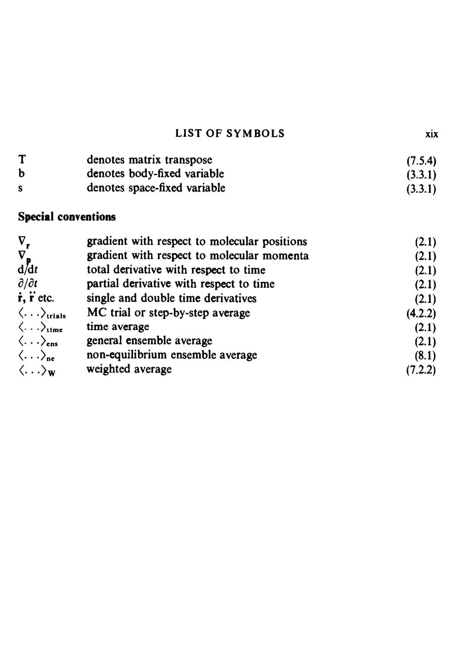
LIST OF SYMBOLS xix T denotes matrix transpose 7.5.4) b denotes body-fixed variable (3.3.1) denotes space-fixed variable (3.3.1) Special conventions 7. gradient with respect to molecular positions 2.1) 。 gradient with respect to molecular momenta (2.1) d/dt total derivative with respect to time (2.1) 8/8t partial derivative with respect to time (2.1) i,ietc. single and double time derivatives (2.1) 〈..)trials MC trial or step-by-step average (4.2.2) (..〉me time average (2.1) 〈.)cns general ensemble average (2.1) (..)ne non-equilibrium ensemble average (8.1) 〈.〉w weighted average (7.2.2)
1 INTRODUCTION 1.1 A short history of computer simulation What is a liquid?As you read this book,you may be mixing up,drinking down, sailing on,or sinking in,a liquid.Liquids flow,although they may be very viscous.They may be transparent,or they may scatter light strongly.Liquids may be found in bulk,or in the form of tiny droplets.They may be vaporized or frozen.Life as we know it probably evolved in the liquid phase,and our bodies are kept alive by chemical reactions occurring in liquids.There are many fascinating details of liquid-like behaviour,covering thermodynamics,struc- ture,and motion.Why do liquids behave like this? The study of the liquid state of matter has a long and rich history,from both the theoretical and experimental standpoints.From early observations of Brownian motion to recent neutron scattering experiments,experimentalists have worked to improve the understanding of the structure and particle dynamics that characterize liquids.At the same time,theoreticians have tried to construct simple models which explain how liquids behave.In this book,we concentrate exclusively on molecular models of liquids,and their analysis by computer simulation.For excellent accounts of the current status of liquid science,the reader should consult the standard references [Barker and Henderson 1976;Rowlinson and Swinton 1982;Hansen and McDonald 1986. Early models of liquids [Morrell and Hildebrand 1936]involved the physical manipulation and analysis of the packing of a large number of gelatine balls,representing the molecules;this resulted in a surprisingly good three-dimensional picture of the structure of a liquid,or perhaps a random glass,and later applications of the technique have been described [Bernal and King 1968].Even today,there is some interest in the study of assemblies of metal ball bearings,kept in motion by mechanical vibration [Pieranski, Malecki,Kuczynski,and Wojciechowski 19787.However,the use of large numbers of physical objects to represent molecules can be very time- consuming,there are obvious limitations on the types of interactions between them,and the effects of gravity can never be eliminated.The natural extension of this approach is to use a mathematical,rather than a physical,model,and to perform the analysis by computer. It is now over 30 years since the first computer simulation of a liquid was carried out at the Los Alamos National Laboratories in the United States [Metropolis,Rosenbluth,Rosenbluth,Teller,and Teller 1953].The Los Alamos computer,called MANIAC,was at that time one of the most powerful available;it is a measure of the recent rapid advance in computer technology that microcomputers of comparable power are now available to the general