216 CHAPTER 10.FUNDAMENTALS OF MIMO FEEDBACK CONTROL y(t)y(t)di (10.1-53) Assume now that the function G(s)is matrin valued with dimension m x n. Then the definition (10.1-52)becomes {10.1-54) where G(s)is in the set Ix of all matrix valued functions of dimension m x n for which (10.1-54)is finite.Equation:10.1-54)cannot be interpreted easily in detemns setin We will discus the implications ateoudervation of the Linear Quadratic Optimal Control problem Let us look next at the linear system y(s)=G:3;uis) and pose the following problern:given a bound onu what is the least upper 10.1-55) bound ony2?In other words.we ar looking for the operator norm induced by·I2- Theorem10l4.Letu∈L好nndG三”Th题yL and the norm of the operator G induced by 1 is Gll=supiG:G 110.1-56) where Giw is the x-norm of ih junion G in the frequency domain. Proof.WVe will sketch the proof for the Sis()c.se (y yu)and leave the rest as an exercise. is后=e=金一nud Thus Hy服≤s This proves thatisan upperboudheduced o To prove that it is in fact the least upper bound and thus ecp:al tothe induced norm we have to show that the bound can be reached for a spcific u.The specific u is a"sinusoid" modified to be square integrable and occurri:g ai the frequency where g()is maximum. 0
10.2.CLASSIC FEEDBACK 217 To appreciate the difference between the 2-norm of an operator and the op- erator norm induced by the 2-norm (oo-norm)we refer the reader back to our discussion of the SISO H2-and He-optimal control problems (Chap.2).We found that for H2-optimal control the performance for a specifc input signal is optimized which implies the minimization of the weighted 2-norm of the sensitiv- ity operator.For H-optimal control the performance for a set of 2-norm bounded signals is optimized.This implies minimization of the norm of the sensitivity op- erator induced by the 2-norm,which we showed io be equal to the -norm of the. sensitivity function (Thm.10.1-) 10.2 Classic Feedback 10.2.1 Definitions The block diagram of a typical classic feedback loop is shown in Fig.10.2-1A. Here C denotes the controller and P the plant trausfer function.The transfer function P describes the effect of the disturbance d on the process output y. Pn symbolizes the measurement device transfer furcrion.The measured variable ym is corrupted by measurement noise n.The controiler determines the process input (manipulated variable)u on the basis of the ror e.The objective of the feedback loop is to keep y close to the reference (setpoint)r. Cor.monly we will nse the simplified block riiagran:in Fig.10.2-1B.Here d denotes the effect of the disturbance on the ou:put.Exact knowledge of the output y is assumed (Pm =1.n =0). 10.2.2 Multivariable Nyquist Criterion Consider the closed loop system in Fig.10.2-13 when P is square (dim u dim y).Let the open loop transfer mnatrix Pisic be described in state space by 主=.1"÷B2e) 110.2-1) y=Cox+Doi-e) 10.2-2) where e=y-r 10.2-3) Combining (10.2-1)-(10.2-3)we obtain
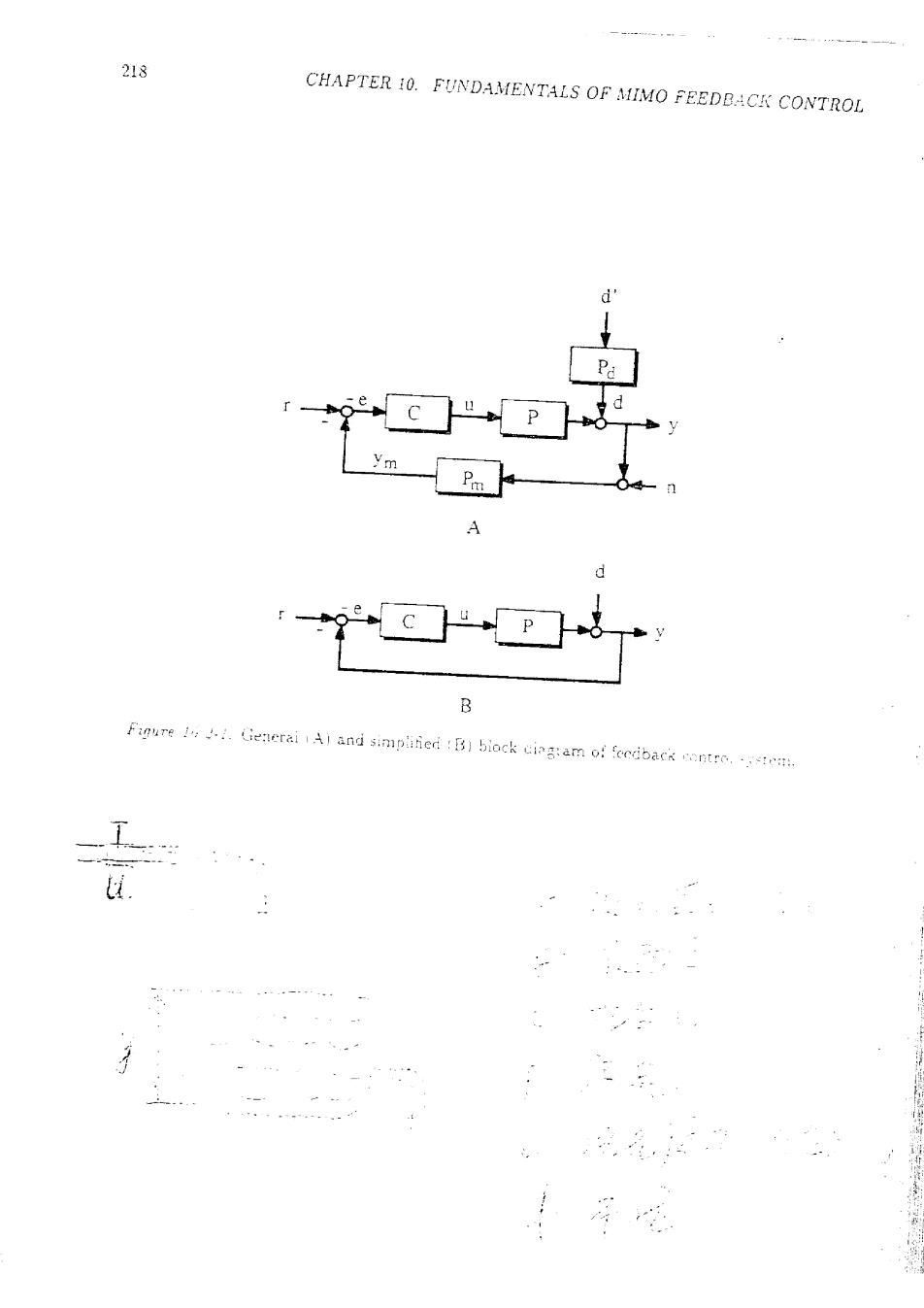
218 CHAPTER 10.FUNDAMENTALS OF MIMO FEEDBACK CONTROL d' ym y B Fiqure :Generai Al and simplifed B)biock ciag:am of fecdback contre
219 10.2.CLASSIC FEEDBACK 10.2-4) 文=Ax+Br (10.2-5) y=Cox+Der where Ae=4。-B(I+D)C。 (10.2-6a) B。=B(I+D)1 10.2-6b) Ce=(I+Do)1C。 (10.2-6c D.=(1+Do)D, 10.2-6d) We define the open-loop characteristic polynomiul (OLCP) ooL det(sI-4o! 10.2-7) and the closed-loop characteristic poiynomial (CLCP] oct=de以sI-Ae 10.2-8) Stabiity is determined by the zeros of the CLCP.We wish to express the CLCP in termns of P(s)C(s).We define the return difference operator F 4 Fs}=I÷P5Co; 10.2-9) and state the following iemma. 引 快 Lemma 10.2-1 (Schur's!formulae for partitioned determinants). Let the square muiriz G be partitioned us Gn G=G2! Gn G22/ Then the determinant can be expressed as detG=dctG1·det(G2-G:GiG:2)if detG:÷Q (10.2-10) -or detG=detG2det(G1-GG2G21》if detG2≠0 (10.2-11)3
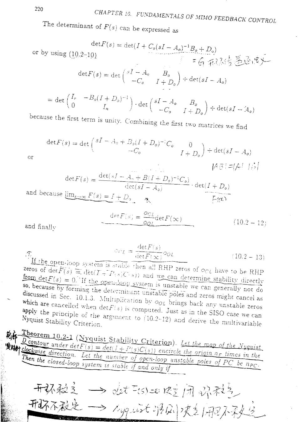
220 CHAPTER 10.FUNDAMENTALS OF MIMO FEEDBACK CONTROL The determinant of F(s)can be expressed as or by using (10.2-10) detF(s)det(I+Co(sI-A0)Be+D.) =6号蒸3,y detF(s)=det -A。 B。 -C。I+D,}÷det(-A) In ÷det(sI-Ao) because the first term is unity.Combining the first two matrices we find deFs到=det(s-i,+,1+DC。0 -Co I+D,÷iet(sl-A) or 4e=!1 detF(s)= det(sI-An+Bi÷D,-iCa ciet(sI-Ao) det(I+Do) and because limF(s)D E) detFis;= OLdetF(x) and Ainallv 90L (10.2-12; 1= detFs) ietFxoL :10.2-13 'If the open-loop system is sablehen a!!RHP zeros of ocL have to be RHP zeros of der F(s)=det(PC))and we can derermine stability directly from detF(s)=0.'If the opeu-loop svsiem is unstable we can generally not do so,because by forming the deter:ninant unstable poles and zeros might cancel as discussed in Sec.10.1.3.Multipiication by oo brings back any unstable zeros which are canceiled when detFs)is computed.Just as in the SISO case we can apply the principle of the argunent to (10.2-12)and derive the multivariable Nyquist Stability Criterion. Theorem 10.2-1 (Nyquist Stability Criterion).the mapofe Vyquist D contour under detFis=det)Cis encircle the origin n tmes in the elockisentheeapnoop poles of PCbep Then the closed-loop sysiem is stlef and onyi 环被3 t5:快/闭彩名 开环不殺是 州庆网照水分