22 INTRODUCTION complete by defining the positions of the sites within the molecule.Normally, these are located at the positions of the nuclei,with the bond lengths obtained from a standard source [CRC 1984]. The site-site Lennard-Jones potentials include an anisotropic dispersion which has the correct r6 radial dependence at long range.However,this is not the exact result for the anisotropic dispersion from second order perturbation theory.The correct formula,in an appropriate functional form for use in a simulation,is given by Burgos,Murthy,and Righini [1982].Its implemen- tation requires an estimate of the polarizability and polarizability anisotropy of the molecule. The most convenient way of representing electrostatic interactions is through partial charges as discussed in Section 1.3.To minimize the calculation of site-site distances,they can be made to coincide with the Lennard-Jones sites,but this is not always desirable or possible;the only physical constraint on partial charge positions is that they should not lie outside the repulsive core region,since the potential might then diverge if molecules came too close.The magnitudes of the charges can be chosen to duplicate the known gas phase electrostatic moments [Gray and Gubbins 1984,Appendix D].Alternatively,the moments may be taken as adjustable parameters.For example,in a simple three-site model of N2 representing only the quadrupole-quadrupole interaction,the best agreement with condensed phase properties is obtained with charges giving a quadrupole 10-15 per cent lower than the gas phase value [Murthy,Singer,Klein,and McDonald 1980]. However,a sensible strategy is to begin with the gas phase values,and alter the repulsive core parameters e and o before changing the partial charges. 1.4.3 Adjusting the model potential The first-guess potential can be used to calculate a number of properties in the gas,liquid,and solid phases;comparison of these results with experiment may be used to refine the potential,and the cycle can be repeated if necessary.The second virial coefficient is given by Bm=-径rd小dan小an,sp(-an.l,)- (1.20) where 4n for a linear molecule and =82 for a non-linear one.This multidimensional integral (four-dimensional for a linear molecule and six- dimensional for a non-linear one)is easily calculated using a non-product algorithm [Murad 1978].Experimental values of B(T)have been compiled by Dymond and Smith [1980].Trial and error adjustment of the Lennard-Jones e and o parameters should be carried out,with any bond lengths and partial charges held fixed,so as to produce the closest match with the experimental
STUDYING SMALL SYSTEMS 23 B(T).This will produce an improved potential,but still one that is based on pair properties. The next step is to carry out a series of computer simulations of the liquid state,as described in Chapters 3 and 4.The densities and temperatures of the simulations should be chosen to be close to the orthobaric curve of the real system,i.e.the liquid-vapour coexistence line.The output from these simulations,particularly the total internal energy and the pressure,may be compared with the experimental values.The coexisting pressures are readily available [Rowlinson and Swinton 1982],and the internal energy can be obtained approximately from the known latent heat of evaporation.The energy parameters e are adjusted to give a good fit to the internal energies along the orthobaric curve,and the length parameters o altered to fit the pressures.If no satisfactory fit is obtained at this stage,the partial charges may be adjusted. Although the solid state is not the province of this book,it offers a sensitive test of any potential model.Using the experimentally observed crystal structure,and the refined potential model,the lattice energy at zero temperature can be compared with the experimental value (remembering to add a correction for quantum zero-point motion).In addition,the lattice parameters corresponding to the minimum energy for the model solid can be compared with the values obtained by diffraction,and also lattice dynamics calculations [Neto,Righini,Califano,and Walmsley 1978]used to obtain phonons,librational modes,and dispersion curves of the model solid.Finally, we can ask if the experimental crystal structure is indeed the minimum energy structure for our potential.These constitute severe tests of our model-building skills. 1.5 Studying small systems 1.5.1 Introduction Computer simulations are usually performed on a small number of molecules, 10 <N<10000.The size of the system is limited by the available storage on the host computer,and,more crucially,by the speed of execution of the program.The time taken for a double loop used to evaluate the forces or potential energy is proportional to N2.Special techniques(see Chapter 5)may reduce this dependence to (N),for very large systems,but the force/energy loop almost inevitably dictates the overall speed,and,clearly,smaller systems will always be less expensive.If we are interested in the properties of a very small liquid drop,or a microcrystal,then the simulation will be straight- forward.The cohesive forces between molecules may be sufficient to hold the system together unaided during the course of a simulation;otherwise our set of N molecules may be confined by a potential representing a container,which prevents them from drifting apart (see Chapter 11).These arrangements
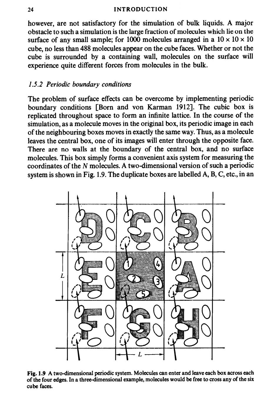
24 INTRODUCTION however,are not satisfactory for the simulation of bulk liquids.A major obstacle to such a simulation is the large fraction of molecules which lie on the surface of any small sample;for 1000 molecules arranged in a 10 x 10 x 10 cube,no less than 488 molecules appear on the cube faces.Whether or not the cube is surrounded by a containing wall,molecules on the surface will experience quite different forces from molecules in the bulk. 1.5.2 Periodic boundary conditions The problem of surface effects can be overcome by implementing periodic boundary conditions [Born and von Karman 1912].The cubic box is replicated throughout space to form an infinite lattice.In the course of the simulation,as a molecule moves in the original box,its periodic image in each of the neighbouring boxes moves in exactly the same way.Thus,as a molecule leaves the central box,one of its images will enter through the opposite face. There are no walls at the boundary of the central box,and no surface molecules.This box simply forms a convenient axis system for measuring the coordinates of the N molecules.A two-dimensional version of such a periodic system is shown in Fig.1.9.The duplicate boxes are labelled A,B,C,etc.,in an Fig.1.9 A two-dimensional periodic system.Molecules can enter and leave each box across each of the four edges.In a three-dimensional example,molecules would be free to cross any of the six cube faces
STUDYING SMALL SYSTEMS 25 arbitrary fashion.As particle 1 moves through a boundary,its images,1A,1B, etc.(where the subscript specifies in which box the image lies)move across their corresponding boundaries.The number density in the central box(and hence in the entire system)is conserved.It is not necessary to store the coordinates of all the images in a simulation (an infinite number!),just the molecules in the central box.When a molecule leaves the box by crossing a boundary,attention may be switched to the image just entering.It is sometimes useful to picture the basic simulation box(in our two-dimensional example)as being rolled up to form the surface of a three-dimensional torus or doughnut,when there is no need to consider an infinite number of replicas of the system,nor any image particles.This correctly represents the topology of the system,if not the geometry.A similar analogy exists for a three-dimensional periodic system,but this is more difficult to visualize! It is important to ask if the properties of a small,infinitely periodic,system, and the macroscopic system which it represents,are the same.This will depend both on the range of the intermolecular potential and the phenomenon under investigation.For a fluid of Lennard-Jones atoms,it should be possible to perform a simulation in a cubic box of side L60,without a particle being able to 'sense'the symmetry of the periodic lattice.If the potential is long ranged (i.e.v(r)~r where v is less than the dimensionality of the system) there will be a substantial interaction between a particle and its own images in neighbouring boxes,and consequently the symmetry of the cell structure is imposed on a fluid which is in reality isotropic.The methods used to cope with long-range potentials,for example in the simulation of charged ions (v(r) r)and dipolar molecules (v(r)~r-3),are discussed in Chapter 5.Recent work has shown that,even in the case of short-range potentials,the periodic boundary conditions can induce anisotropies in the fluid structure [Mandell 1976;Impey,Madden,and Tildesley 1981].These effects are pronounced for small system sizes(N100)and for properties such as the g2 light scattering factor(see Chapter 2),which has a substantial long-range contribution.Pratt and Haan [1981]have developed theoretical methods for investigating the effects of boundary conditions on equilibrium properties. The use of periodic boundary conditions inhibits the occurrence of long- wavelength fluctuations.For a cube of side L,the periodicity will suppress any density waves with a wavelength greater than L.Thus,it would not be possible to simulate a liquid close to the gas-liquid critical point,where the range of critical fluctuations is macroscopic.Furthermore,transitions which are known to be first order often exhibit the characteristics of higher order transitions when modelled in a small box because of the suppression of fluctuations. Examples are the nematic to isotropic transition in liquid crystals [Luckhurst and Simpson 1982]and the solid to plastic crystal transition for N2 adsorbed on graphite [Mouritsen and Berlinsky 1982].The same limitations apply to the simulation of long-wavelength phonons in model solids,where,in addition, the cell periodicity picks out a discrete set of available wave-vectors (i.e
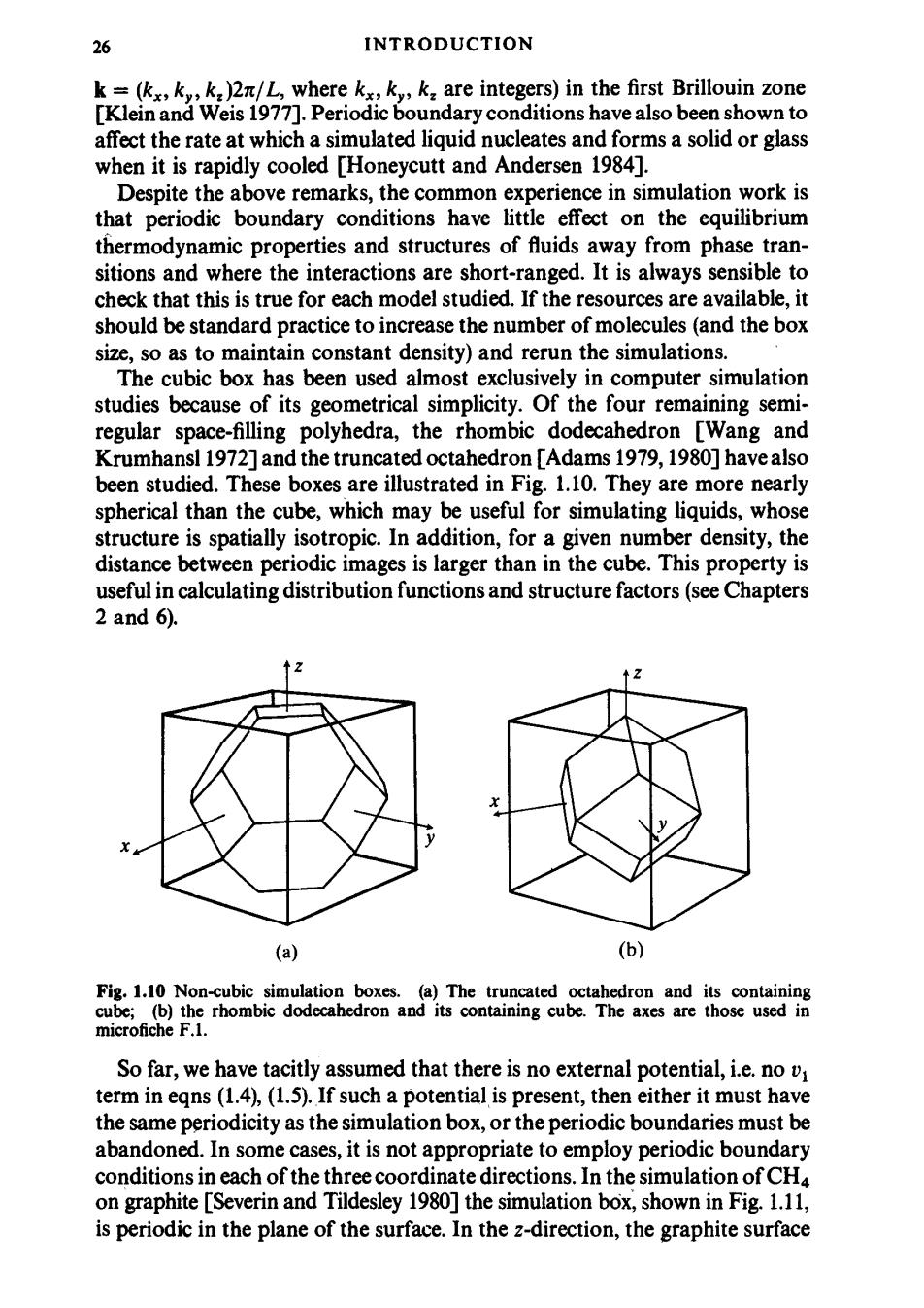
26 INTRODUCTION k=(kx,ky,k:)2n/L,where kx,k,k:are integers)in the first Brillouin zone [Klein and Weis 1977].Periodic boundary conditions have also been shown to affect the rate at which a simulated liquid nucleates and forms a solid or glass when it is rapidly cooled [Honeycutt and Andersen 1984]. Despite the above remarks,the common experience in simulation work is that periodic boundary conditions have little effect on the equilibrium thermodynamic properties and structures of fluids away from phase tran- sitions and where the interactions are short-ranged.It is always sensible to check that this is true for each model studied.If the resources are available,it should be standard practice to increase the number of molecules (and the box size,so as to maintain constant density)and rerun the simulations. The cubic box has been used almost exclusively in computer simulation studies because of its geometrical simplicity.Of the four remaining semi- regular space-filling polyhedra,the rhombic dodecahedron [Wang and Krumhansl 1972]and the truncated octahedron [Adams 1979,1980]have also been studied.These boxes are illustrated in Fig.1.10.They are more nearly spherical than the cube,which may be useful for simulating liquids,whose structure is spatially isotropic.In addition,for a given number density,the distance between periodic images is larger than in the cube.This property is useful in calculating distribution functions and structure factors(see Chapters 2 and 6). (a) (b) Fig.1.10 Non-cubic simulation boxes.(a)The truncated octahedron and its containing cube;(b)the rhombic dodecahedron and its containing cube.The axes are those used in microfiche F.1. So far,we have tacitly assumed that there is no external potential,i.e.no v term in eqns(1.4),(1.5).If such a potential is present,then either it must have the same periodicity as the simulation box,or the periodic boundaries must be abandoned.In some cases,it is not appropriate to employ periodic boundary conditions in each of the three coordinate directions.In the simulation of CH4 on graphite [Severin and Tildesley 1980]the simulation box,shown in Fig.1.11, is periodic in the plane of the surface.In the z-direction,the graphite surface