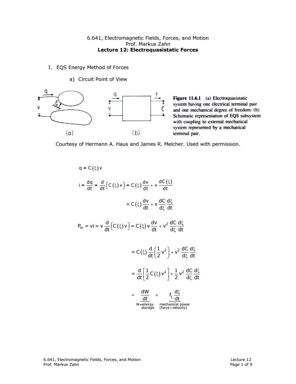
6.641,Electromagnetic Fields,Forces,and Motion Prof.Markus Zahn Lecture 12:Electroquasistatic Forces I.EQS Energy Method of Forces a)Circuit Point of View Figure 11.6.1 (a)Electroquasistatic system having one electrical terminal pair and one mechanical degree of freedom.(b) Schematic representation of EQS subsystem with coupling to extemal mechanical system represented by a mechanical (a) (b) terminal pair. Courtesy of Hermann A.Haus and James R.Melcher.Used with permission. q=C()v i-=品[cey]-ce0+vace dt =c附0+ve da dt R=m=v是[c(y-c张+E架 d dt =ce是va d dt -Bce +1v2 dc d d dt dw d dt W=energy mechanical power storage (force x velocity) 6.641,Electromagnetic Fields,Forces,and Motion Lecture 12 Prof.Markus Zahn Page 1 of 9
6.641, Electromagnetic Fields, Forces, and Motion Lecture 12 Prof. Markus Zahn Page 1 of 9 6.641, Electromagnetic Fields, Forces, and Motion Prof. Markus Zahn Lecture 12: Electroquasistatic Forces I. EQS Energy Method of Forces a) Circuit Point of View Courtesy of Hermann A. Haus and James R. Melcher. Used with permission. q=C v ( ) ξ () () (ξ) ⎡ ⎤ ξ ξ+ ⎣ ⎦ dq d dv dC i= = C v =C v dt dt dt dt ( ) ξ ξ + ξ dv dC d =C v dt d dt ( ) ⎛ ⎞ ξ ξ + ⎜ ⎟ ⎝ ⎠ ξ d 1 dC d 2 2 =C v v dt 2 d dt ( ) ⎡ ⎤ ξ ξ + ⎢ ⎥ ⎣ ⎦ ξ d 1 1 dC d 2 2 = Cv v dt 2 2 d dt N N W energy mechanical power storage (force velocity) dW d f dt dt ξ = × ξ = + () () ξ ⎡ ⎤ ξ ξ+ ⎣ ⎦ ξ 2 in d dv P = vi = v C v = C v v dt dt d dt dC d
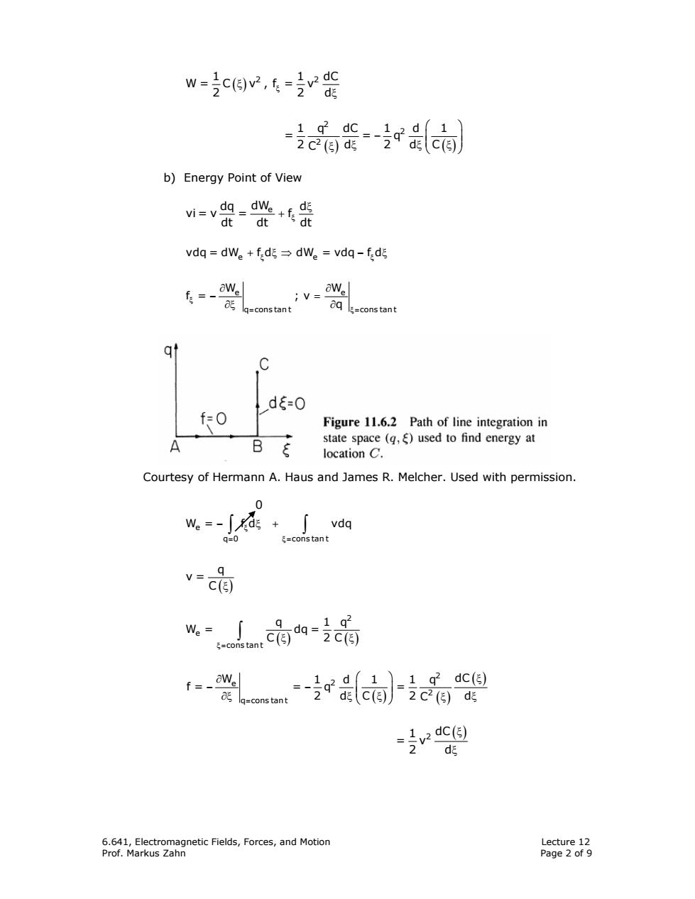
w=2c旧,6- -cge=r{c 2c2()d店 dEc佰 b)Energy Point of View n=v-0+e能 dt dt vdq=dWe +f:d=dWe vdq-fd -、w/ a=constant ;v=w 6q l=cons tant C dξ=0 f=0 Figure 11.6.2 Path of line integration in A Bξ state space (g,E)used to find energy at location C. Courtesy of Hermann A.Haus and James R.Melcher.Used with permission. 0 w。=-∫d+ vdq q=0 E=cons tant v=0 w.=c间 =cons tant q dq=2C(E) 1q2 f=-oW/ 1q2dc(5) g=constant 2 C2()dE v dc() d 6.641,Electromagnetic Fields,Forces,and Motion Lecture 12 Prof.Markus Zahn Page 2 of 9
6.641, Electromagnetic Fields, Forces, and Motion Lecture 12 Prof. Markus Zahn Page 2 of 9 ( ) ξ ξ ξ 1 1 2 2 dC W= C v , f = v 2 2 d ( ) ( ) ⎛ ⎞ − ⎜ ⎟ ξ ξ ξ ⎜ ⎟ ξ ⎝ ⎠ 2 2 2 1 q dC 1 d 1 = =q 2 d 2 dC C b) Energy Point of View ξ ξ + dq dWe d vi = v = f dt dt dt ξ ξ + ξ⇒ − ξ vdq = dW f d dW = vdq f d e e ξ = ξ= ∂ ∂ − = ∂ξ ∂ e e q cons tan t cons tan t W W f = ; v q Courtesy of Hermann A. Haus and James R. Melcher. Used with permission. 0 ξ = ξ= − ξ+ e ∫ ∫ q 0 cons tan t W = f d vdq ( ) ξ q v = C ( ) ( ) ξ = ξ ξ ∫ 2 e cons tan t q 1q W = dq = C C 2 (ξ) ξ 2 1 dC = v 2 d ( ) ( ) ( ) = ∂ ⎛ ⎞ ξ − − ⎜ ⎟ ∂ξ ξ ⎜ ⎟ ξ ξ ξ ⎝ ⎠ 2 e 2 2 q cons tan t W 1 d 1 1q dC f = = q = 2d 2 d C C
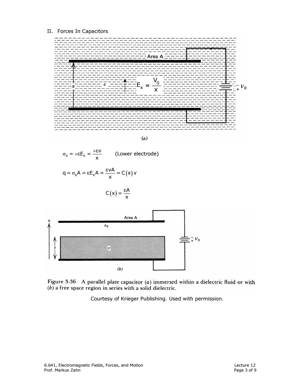
II.Forces In Capacitors Area A e二3 (a) 0s=+8Ex=-+8y (Lower electrode) X q=cA=EEA=SVA =C(x)v C(x)=A X Area A Eo Vo (b) Figure 3-36 A parallel plate capacitor(a)immersed within a dielectric fluid or with (b)a free space region in series with a solid dielectric. Courtesy of Krieger Publishing.Used with permission. 6.641,Electromagnetic Fields,Forces,and Motion Lecture 12 Prof.Markus Zahn Page 3 of 9
6.641, Electromagnetic Fields, Forces, and Motion Lecture 12 Prof. Markus Zahn Page 3 of 9 II. Forces In Capacitors s x v = E= x + σ + ε ε (Lower electrode) σ ( ) ε ε s x vA q= A= E A= =C x v x ( ) εA Cx= x Courtesy of Krieger Publishing. Used with permission. Ex = V0 x

a)Coulombic force method on upper electrode: 反=,EA=-EA=- A 2 2x2 2 because E in electrode=0,E outside electrode Ex -Take average Energy method:C(x)=SA X 器或终装 2 xZ EZAZ 2EA b) area A lE。 Figure 11.6.3 Specific example of EQS b systems having one electrical and one 0 mechanical terminal pair. Courtesy of Hermann A.Haus and James R.Melcher.Used with permission. =5b EA+EA =e5+8b EE0A 6-}部 1 6-r品c--2et的 三一 (e5+8ob2 6.641,Electromagnetic Fields,Forces,and Motion Lecture 12 Prof.Markus Zahn Page 4 of 9
6.641, Electromagnetic Fields, Forces, and Motion Lecture 12 Prof. Markus Zahn Page 4 of 9 a) Coulombic force method on upper electrode: σ− − ε ε 2 2 x sx x 2 1 1 1v f = E A= E A= A 2 22 x 1 2 because E in electrode=0, E outside electrode = Ex Take average Energy method: ( ) εA Cx= x ⎛ ⎞ − ⎜ ⎟ ⎝ ⎠ ε ε 2 2 2 x 2 1 dC 1 d 1 1 v A f= v = v A = 2 dx 2 dx x 2 x ( ) ⇒ − ε ε x q qx 1 v= = f = C x A 2 A 2 x 2 2 q x ε2 2 A − ε 2 1 q = 2 A b) Courtesy of Hermann A. Haus and James R. Melcher. Used with permission. ( ) + ξ ξ ε0 ε a b a b 1 11 A A = ;C = ,C = C CC b ξ + ε ε 0 b = A A ε ε ξ + ε ε 0 0 b = A ( ) ξ ( ) − ⎛ ⎞ − − ⎜ ⎟ ξ ξ ⎜ ⎟ ξ ⎝ ⎠ εξ+ε ε ε ε 2 2 2 0 0 0 1 q = q = b= 1 d 1 d 1q 2 2 d Ad 2 A C f ( ) ( ) ( ) ξ ⎡ ⎤ ξ − ⎢ ⎥ ξ ξ ⎣ ⎦ εε ε ε εξ+ε εξ+ε 2 2 2 2 0 0 2 0 0 1d 1d 1 A vA =v C =v = 2d 2d b 2 b f
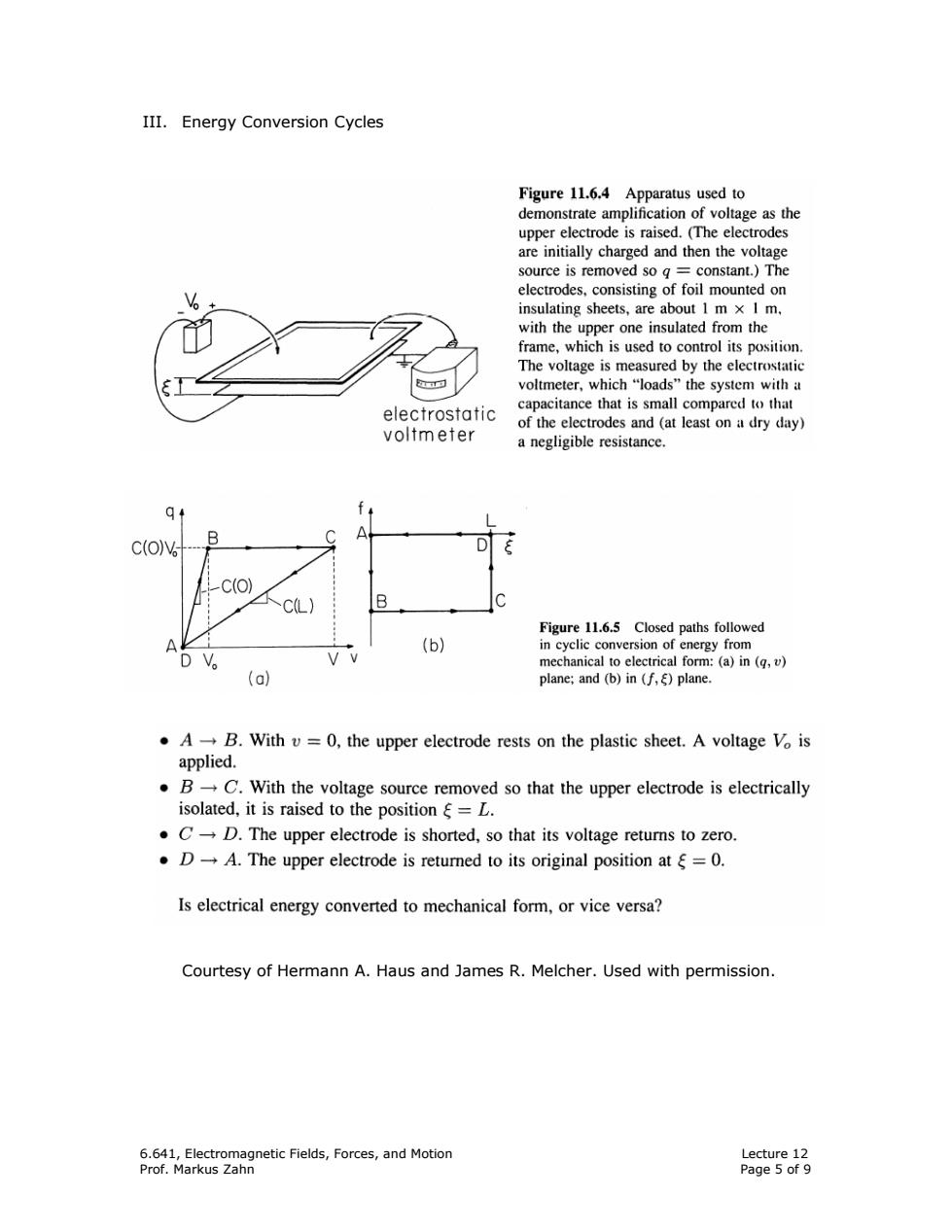
III.Energy Conversion Cycles Figure 11.6.4 Apparatus used to demonstrate amplification of voltage as the upper electrode is raised.(The electrodes are initially charged and then the voltage source is removed so g constant.)The electrodes,consisting of foil mounted on insulating sheets,are about 1 m x I m. with the upper one insulated from the frame,which is used to control its position. The voltage is measured by the electrostatic voltmeter,which“loads'”the system with a electrostatic capacitance that is small compared to that of the electrodes and (at least on a dry day) voltmeter a negligible resistance. B C(OV -C(O) C(L) B Figure 11.6.5 Closed paths followed A (b) in cyclic conversion of energy from DV mechanical to electrical form:(a)in(q,v) (a) plane;and (b)in (f,)plane. .A-B.With v=0,the upper electrode rests on the plastic sheet.A voltage Vo is applied. B-C.With the voltage source removed so that the upper electrode is electrically isolated,it is raised to the position =L. .C-D.The upper electrode is shorted,so that its voltage returns to zero. ·D→A.The upper electrode is retured to its original position atξ=O. Is electrical energy converted to mechanical form,or vice versa? Courtesy of Hermann A.Haus and James R.Melcher.Used with permission. 6.641,Electromagnetic Fields,Forces,and Motion Lecture 12 Prof.Markus Zahn Page 5 of 9
6.641, Electromagnetic Fields, Forces, and Motion Lecture 12 Prof. Markus Zahn Page 5 of 9 III. Energy Conversion Cycles Courtesy of Hermann A. Haus and James R. Melcher. Used with permission