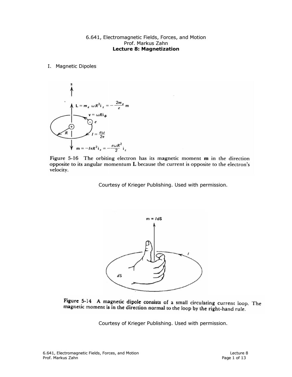
6.641,Electromagnetic Fields,Forces,and Motion Prof.Markus Zahn Lecture 8:Magnetization I.Magnetic Dipoles 木L=m。wR12=-2mm e v=wRi中 R 21= ew 2n Figure 5-16 The orbiting electron has its magnetic moment m in the direction opposite to its angular momentum L because the current is opposite to the electron's velocity. Courtesy of Krieger Publishing.Used with permission. m =/ds Figure 5-14 A magnetic dipole consists of a small circulating current loop.The magnetic moment is in the direction normal to the loop by the right-hand rule. Courtesy of Krieger Publishing.Used with permission. 6.641,Electromagnetic Fields,Forces,and Motion Lecture 8 Prof.Markus Zahn Page 1 of 13
6.641, Electromagnetic Fields, Forces, and Motion Lecture 8 Prof. Markus Zahn Page 1 of 13 6.641, Electromagnetic Fields, Forces, and Motion Prof. Markus Zahn Lecture 8: Magnetization I. Magnetic Dipoles Courtesy of Krieger Publishing. Used with permission. Courtesy of Krieger Publishing. Used with permission
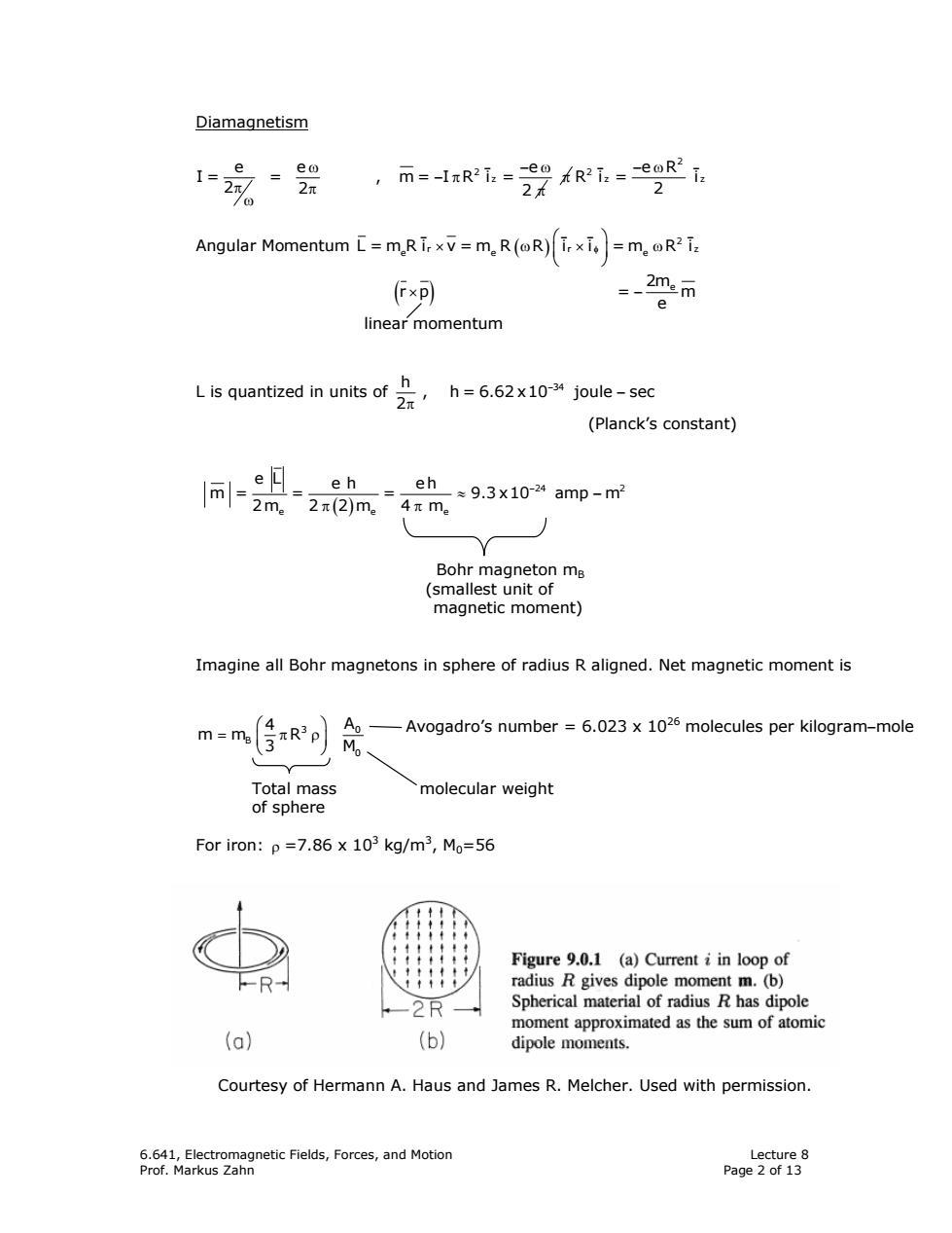
Diamagnetism e 1=2 eo 2元 ,me1R2i.=22R2i=e9Ri /0 Angular Momentum [=mRi,x=mR(R)x=mR, (Fxp) 、 2mem e linear momentum L is quantized in units of h=6.62x10⁻³⁴ joule-sec 2π (Planck's constant) e且- m=2m eh eh≈9.3x10⁻²⁴amp-m2 2π(2)m。4πme Bohr magneton ms (smallest unit of magnetic moment) Imagine all Bohr magnetons in sphere of radius R aligned.Net magnetic moment is m=me 台aRp Ao Avogadro's number 6.023 x 1026 molecules per kilogram-mole M Total mass molecular weight of sphere For iron:p =7.86 x 10³ kg/m3,Mo=56 Figure 9.0.1 (a)Current i in loop of -R radius R gives dipole moment m.(b) 2R Spherical material of radius R has dipole moment approximated as the sum of atomic (a) (b) dipole moments Courtesy of Hermann A.Haus and James R.Melcher.Used with permission. 6.641,Electromagnetic Fields,Forces,and Motion Lecture 8 Prof.Markus Zahn Page 2 of 13
6.641, Electromagnetic Fields, Forces, and Motion Lecture 8 Prof. Markus Zahn Page 2 of 13 Diamagnetism Angular Momentum ( ) _ __ _ 2 r rz L=mRi v=m R R i i =m R i ee e φ ⎛ ⎞ × ω× ω ⎜ ⎟ ⎝ ⎠ (r p× ) = m 2me e − linear momentum L is quantized in units of h 34 , h = 6.62 x10 joule sec 2 − − π (Planck’s constant) Bohr magneton mB (smallest unit of magnetic moment) Imagine all Bohr magnetons in sphere of radius R aligned. Net magnetic moment is 3 0 B 0 4 A mm R 3 M ⎛ ⎞ = πρ ⎜ ⎟ ⎝ ⎠ Total mass molecular weight of sphere For iron: ρ =7.86 x 10³ kg/m3 , M0=56 Courtesy of Hermann A. Haus and James R. Melcher. Used with permission. Avogadro’s number = 6.023 x 1026 molecules per kilogram−mole ω − ω − π π π π ω _ 2 z e e e I= = , m= I R i = 2 2 2 π − ω _ 2 _ 2 z z e R Ri= i 2 ( ) − ≈ − 24 9.3 x10 amp π π 2 e ee e L e h eh m= = = m 2m 2 2 m 4 m
For a current loop m=izR2=m专R2p先 ,Ao→i=m3 }7.8610 6.023×1026 ForR=10cm→i=9.3×10² 56 1.05 x 10⁵ Amperes Thus,an ordinary piece of iron can have the same magnetic moment as a current loop of radius 10 cm of 105 Amperes current. B.Magnetic Dipole Field H=Hom 2cos0ir+sin0io 4πr30 (multiply top bottom by Ho) Electric Dipole Field E= 2cos0 ir+sin0 io 4πc.r3 Analogy p→μom P=Np=M=Nm,N =of magnetic dipoles/volume 1 Polarization Magnetization II.Maxwell's Equations with Magnetization EQS MOS (e目)=pu-V.p 7.(可=-7(闪 Po=-V.P(Polarization or paired Pm=-V.(Ho M)(magnetic charge charge density) density) n[旧-E门=-n[F-p]+如 n[,-f】=-n[你-)】 6.641,Electromagnetic Fields,Forces,and Motion Lecture 8 Prof.Markus Zahn Page 3 of 13
6.641, Electromagnetic Fields, Forces, and Motion Lecture 8 Prof. Markus Zahn Page 3 of 13 For a current loop 2 3 0 0 B B 0 0 4 4 A A m=i R =m R i=m R 3 M 3M π πρ ⇒ ρ For R = 10 cm ( ) ⎛ ⎞ ( × ) ⇒× × ⎜ ⎟ ⎝ ⎠ 26 -24 3 4 6.023 10 i = 9.3 10 .1 7.86 10 3 56 = 1.05 x 10⁵ Amperes Thus, an ordinary piece of iron can have the same magnetic moment as a current loop of radius 10 cm of 105 Amperes current. B. Magnetic Dipole Field _ _ 0 r 3 0 m H = 2 cos i sin i 4 r θ µ ⎡ ⎤ θ+ θ ⎢ ⎥ π µ ⎣ ⎦ (multiply top & bottom by µ0 ) Electric Dipole Field θ ⎡ ⎤ θ+ θ ⎢ ⎥ π ε ⎣ ⎦ _ _ r 3 0 p E = 2 cos i sin i 4 r Analogy p m → µ0 P = Np M = Nm ⇒ , N = # of magnetic dipoles / volume Polarization Magnetization II. Maxwell’s Equations with Magnetization EQS ∇ ρ− i i ( ) ε0 u E= P ∇ ρ −∇ i p = P (Polarization or paired charge density) ( ) ⎡ ⎤ ⎡ ⎤ − − −+ ⎢ ⎥ ⎣ ⎦ ⎢ ⎥ ⎣ ⎦ i i ε α b a b n E E =n P P 0 s σ u MQS ∇ − i i (µ0 0 H= M ) ∇ µ( ) ρ −∇ µ m = i( 0 M) (magnetic charge density) ( ) ( ) α b a b n H H =n M M 0 0 ⎡ ⎤⎡ ⎤ − −µ − ⎢ ⎥⎢ ⎥ ⎣ ⎦⎣ ⎦ i i µ
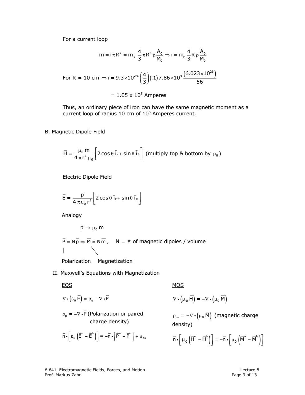
0p=-n[p-p] cm=-n你-] VxH-j xE-品h何+网 MOS Equations B=(H+M)Magnetic flux density B has units of Teslas(1 Tesla =10,000 Gauss) 7.B=0 n[6-B]=0 VxE-_0B Γat vxH=j (total fiux) III.Magnetic Field Intensity along Axis of a Uniformly Magnetized Cylinder d/2 H: d/2 R Figure 9.3.1 (a)Cylinder of circular cross-section uniformly magnetized in the direction of its axis.(b)Axial distribution of scalar magnetic potential and(c)axial magnetic field intensity.For these distributions,the cylinder length is assumed to be equal to its diameter. 6.641,Electromagnetic Fields,Forces,and Motion Lecture 8 Prof.Markus Zahn Page 4 of 13
6.641, Electromagnetic Fields, Forces, and Motion Lecture 8 Prof. Markus Zahn Page 4 of 13 ( ) a b sm 0 =n M M ⎡ ⎤ σ −µ − ⎢ ⎥ ⎣ ⎦ i ∇ ×H=J ( ) ∂ ∇× − µ + ∂ E= H M 0 t MQS Equations B= H M µ + 0 ( ) Magnetic flux density B has units of Teslas (1 Tesla = 10,000 Gauss) ∇ = iB 0 a a n B B =0 ⎡ ⎤ − ⎢ ⎥ ⎣ ⎦ i B E = t ∂ ∇× − ∂ ∇ × H=J III. Magnetic Field Intensity along Axis of a Uniformly Magnetized Cylinder ⎡ ⎤ σ− − ⎢ ⎥ ⎣ ⎦ i a b sp =n P P λ λ ∫ i S d v = , = B da dt (total flux)
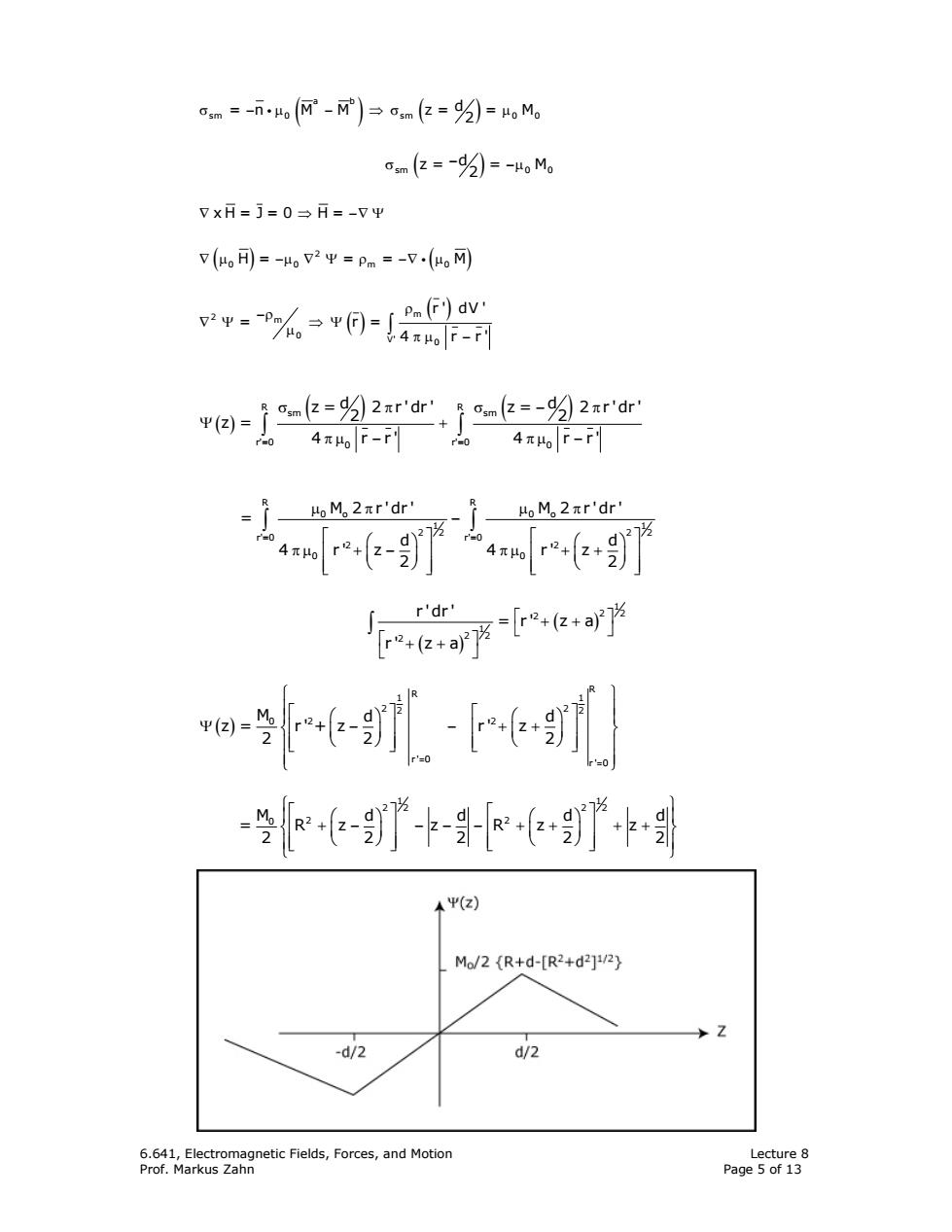
om=-n网-)→m亿=2)=,Mg om(2=-5)=-oM。 7xH=j=0→H=-VΨ 7(可=-2平=pm=-7.( - 驰了a-2rs的2ro 4πoF-r 二+ 4元4oF-r oM。2πr'dr e o-egp -登- Ψ(z) Mo/2{R+d-[R2+d2]2} -d/2 d/2 6.641,Electromagnetic Fields,Forces,and Motion Lecture 8 Prof.Markus Zahn Page 5 of 13
6.641, Electromagnetic Fields, Forces, and Motion Lecture 8 Prof. Markus Zahn Page 5 of 13 ⎧ ⎫ ⎡ ⎤⎡ ⎤ ⎪ ⎪ ⎛⎞ ⎛⎞ ⎨ ⎬ ⎢ ⎥⎢ ⎥ + − −− − + + ++ ⎜⎟ ⎜⎟ ⎪ ⎪ ⎝⎠ ⎝⎠ ⎣ ⎦⎣ ⎦ ⎩ ⎭ 1 1 2 2 2 2 M0 2 2 dd dd = Rz z Rz z 2 22 22 σ − µ − ⇒σ µ i ( ) ( ) a b sm 0 sm 0 0 = n M M z= = M d 2 ( ) σ − − sm 0 0 z= = M d 2 µ ∇ ⇒ xH= J=0 H= −∇ Ψ ∇ µ −µ ∇ Ψ ρ −∇ µ ( ) i( ) 2 00 m 0 H= = = M ( ) −ρ ρ ( ) ∇ Ψ ⇒Ψ µ πµ − ∫ 2 m m 0 V' 0 r ' dV ' = r = 4 r r' ( ) σ π σ −π ( ) ( ) Ψ + πµ − πµ − ∫ ∫ R R sm sm r'=0 0 0 r'=0 z = 2 r ' dr ' z = 2 r ' dr ' d d 2 2 z = 4 r r' 4 r r' µ π µ π − ⎡⎤ ⎡ ⎛ ⎞ ⎛ ⎞ πµ + − ⎢⎥ ⎢ πµ + + ⎜ ⎟ ⎜ ⎟ ⎝ ⎠ ⎝ ⎠ ⎣⎦ ⎣ ∫ ∫ R R 0 o 0 o 1 1 2 2 2 2 r'=0 r'=0 2 2 0 0 M 2 r ' dr ' M 2 r ' dr ' = d d 4 r' z 4 r' z 2 2 ⎤ ⎥ ⎥⎦ ( ) ( ) ⎡ + + ⎤ ⎣ ⎦ ⎡ ⎤ + + ⎣ ⎦ ∫ 1 2 2 2 1 2 2 2 r ' dr ' = r' z a r' z a ( ) = = ⎧ ⎫ ⎪ ⎪ ⎡ ⎤⎡ ⎤ ⎛ ⎞ ⎛ ⎞ Ψ −− ⎨ ⎬ ⎢ ⎥⎢ ⎥ + + ⎜ ⎟ ⎜ ⎟ ⎪ ⎪ ⎢ ⎥⎢ ⎥ ⎝ ⎠ ⎝ ⎠ ⎣ ⎦⎣ ⎦ ⎩ ⎭ R R 1 1 2 2 2 2 0 2 2 r' 0 r' 0 M d d z = r' + z r' z 2 2 2