Chapter 13 Maxwell's Equations and Electromagnetic Waves 13.1 The Displacement Current................. 13-3 13.2 Gauss's Law for Magnetism........ 13-5 13.3 Maxwell's Equations............... 13-6 13.4 Plane Traveling Electromagnetic Waves....... 13-7 13.4.1 One-Dimensional Wave Equation... 13-12 13.4.2 Gaussian One Dimensional Wave Pulse 13-13 13.5 Standing Electromagnetic Waves.................. 13-18 13.6 Poynting Vector… 13-21 Example 13.1:Solar Constant................ 13-23 Example 13.2:Intensity of a Standing Wave............ 13-24 13.6.1 Energy Transport...... 13-25 13.6.2 Power flow in a Solenoid with Changing Current 13-26 13.7 Momentum and Radiation Pressure...................... 13-28 13.8 Production of Electromagnetic Waves........... 13-29 13.8.1 Electric Dipole Radiation Movie....... 13-31 13.8.2 Another Electric Dipole Radiation Movie..... 13-31 13.8.3 Radiation From a Quarter-Wave Antenna Animation...............13-32 13.8.4 Plane Waves.… 13-32 13.8.5 Sinusoidal Electromagnetic Wave.................. 13-37 13.9 Summary 13-39 13.10 Appendix:Reflection of Electromagnetic Waves at Conducting Surfaces..13-41 13.11 Problem-Solving Strategy:Traveling Electromagnetic Waves..........13-46 13.12 Solved Problems............ 13-47 13.12.1 plane Electromagnetic Wave. 13-47 13.12.2 One-Dimensional Wave Equation......... 13-48 13.12.3 Poynting Vector of a Charging Capacitor.... 13-49 13-1
13-1 Chapter 13 Maxwell’s Equations and Electromagnetic Waves 13.1 The Displacement Current.............................................................................. 13-3 13.2 Gauss’s Law for Magnetism........................................................................... 13-5 13.3 Maxwell’s Equations ...................................................................................... 13-6 13.4 Plane Traveling Electromagnetic Waves........................................................ 13-7 13.4.1 One-Dimensional Wave Equation ......................................................... 13-12 13.4.2 Gaussian One Dimensional Wave Pulse................................................ 13-13 13.5 Standing Electromagnetic Waves................................................................. 13-18 13.6 Poynting Vector............................................................................................ 13-21 Example 13.1: Solar Constant.............................................................................. 13-23 Example 13.2: Intensity of a Standing Wave....................................................... 13-24 13.6.1 Energy Transport ................................................................................... 13-25 13.6.2 Power flow in a Solenoid with Changing Current................................. 13-26 13.7 Momentum and Radiation Pressure.............................................................. 13-28 13.8 Production of Electromagnetic Waves ......................................................... 13-29 13.8.1 Electric Dipole Radiation Movie ........................................................... 13-31 13.8.2 Another Electric Dipole Radiation Movie ............................................. 13-31 13.8.3 Radiation From a Quarter-Wave Antenna Animation........................... 13-32 13.8.4 Plane Waves........................................................................................... 13-32 13.8.5 Sinusoidal Electromagnetic Wave ......................................................... 13-37 13.9 Summary....................................................................................................... 13-39 13.10 Appendix: Reflection of Electromagnetic Waves at Conducting Surfaces.. 13-41 13.11 Problem-Solving Strategy: Traveling Electromagnetic Waves.................... 13-46 13.12 Solved Problems ........................................................................................... 13-47 13.12.1 Plane Electromagnetic Wave................................................................. 13-47 13.12.2 One-Dimensional Wave Equation......................................................... 13-48 13.12.3 Poynting Vector of a Charging Capacitor............................................. 13-49
13.12.4 Poynting Vector of a Conductor. 13-51 13.13 Conceptual Questions13-53 13.14 Additional Problems. 13-53 13.14.I Solar Sailing. 3-53 13.142 Reflections ofTrue Love.13-53 13.14.3 Coaxial Cable and Power Flow..... 13-54 13.14.4 Superposition of Electromagnetic Waves............................................1.3-55 13.14.5 Sinusoidal Electromagnetic Wave........ 13-55 13.14.6 Radiation Pressure of Electromagnetic Wave................................... 13-55 13.14.7 Energy of Electromagnetic Waves..... 13-56 13.14.8 Wave Equation. 13-56 13.14.9 Electromagnetic Plane Wave........................ 13-56 13.14.10 Sinusoidal Electromagnetic Wave........................ 13-57 13.15 Generating Plane Electromagnetic Waves Simulation............. 13-58 13-2
13-2 13.12.4 Poynting Vector of a Conductor............................................................ 13-51 13.13 Conceptual Questions ................................................................................... 13-53 13.14 Additional Problems ..................................................................................... 13-53 13.14.1 Solar Sailing .......................................................................................... 13-53 13.14.2 Reflections of True Love....................................................................... 13-53 13.14.3 Coaxial Cable and Power Flow............................................................. 13-54 13.14.4 Superposition of Electromagnetic Waves ............................................. 13-55 13.14.5 Sinusoidal Electromagnetic Wave......................................................... 13-55 13.14.6 Radiation Pressure of Electromagnetic Wave ....................................... 13-55 13.14.7 Energy of Electromagnetic Waves........................................................ 13-56 13.14.8 Wave Equation ...................................................................................... 13-56 13.14.9 Electromagnetic Plane Wave................................................................. 13-56 13.14.10Sinusoidal Electromagnetic Wave......................................................... 13-57 13.15 Generating Plane Electromagnetic Waves Simulation ................................. 13-58
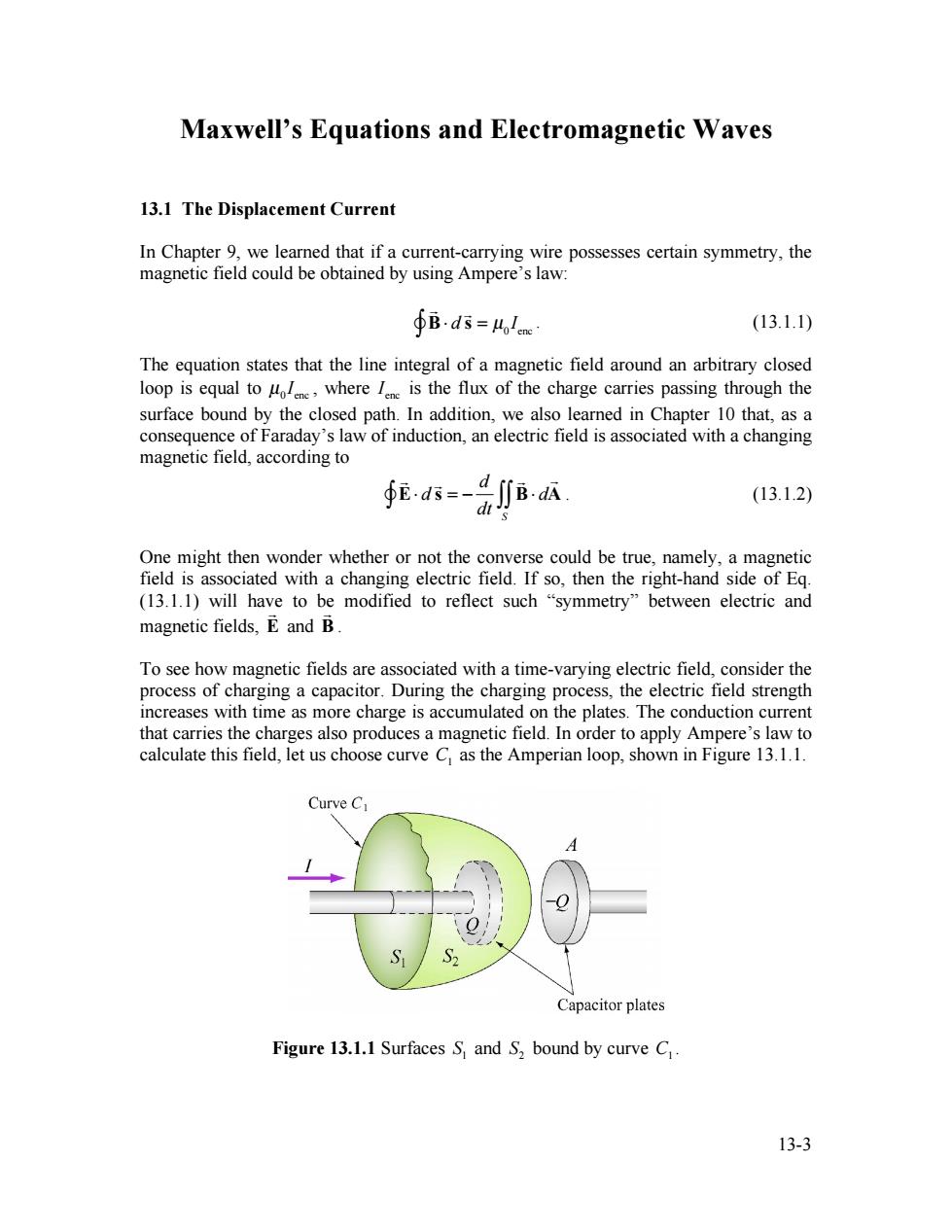
Maxwell's Equations and Electromagnetic Waves 13.1 The Displacement Current In Chapter 9,we learned that if a current-carrying wire possesses certain symmetry,the magnetic field could be obtained by using Ampere's law: Bds=Molcne (13.1.1) The equation states that the line integral of a magnetic field around an arbitrary closed loop is equal to ol where I is the flux of the charge carries passing through the surface bound by the closed path.In addition,we also learned in Chapter 10 that,as a consequence of Faraday's law of induction,an electric field is associated with a changing magnetic field,according to (13.1.2) One might then wonder whether or not the converse could be true,namely,a magnetic field is associated with a changing electric field.If so,then the right-hand side of Eq. (13.1.1)will have to be modified to reflect such "symmetry"between electric and magnetic fields,E and B To see how magnetic fields are associated with a time-varying electric field,consider the process of charging a capacitor.During the charging process,the electric field strength increases with time as more charge is accumulated on the plates.The conduction current that carries the charges also produces a magnetic field.In order to apply Ampere's law to calculate this field,let us choose curve C as the Amperian loop,shown in Figure 13.1.1. Curve C Capacitor plates Figure 13.1.1 Surfaces S and S,bound by curve C 13-3
13-3 Maxwell’s Equations and Electromagnetic Waves 13.1 The Displacement Current In Chapter 9, we learned that if a current-carrying wire possesses certain symmetry, the magnetic field could be obtained by using Ampere’s law: ! B! d ! s "" = µ0 Ienc . (13.1.1) The equation states that the line integral of a magnetic field around an arbitrary closed loop is equal to 0 enc µ I , where enc I is the flux of the charge carries passing through the surface bound by the closed path. In addition, we also learned in Chapter 10 that, as a consequence of Faraday’s law of induction, an electric field is associated with a changing magnetic field, according to ! E! d ! s "" = # d dt ! B! d ! A S "" . (13.1.2) One might then wonder whether or not the converse could be true, namely, a magnetic field is associated with a changing electric field. If so, then the right-hand side of Eq. (13.1.1) will have to be modified to reflect such “symmetry” between electric and magnetic fields, E ! and B ! . To see how magnetic fields are associated with a time-varying electric field, consider the process of charging a capacitor. During the charging process, the electric field strength increases with time as more charge is accumulated on the plates. The conduction current that carries the charges also produces a magnetic field. In order to apply Ampere’s law to calculate this field, let us choose curve C1 as the Amperian loop, shown in Figure 13.1.1. Figure 13.1.1 Surfaces 1 S and 2 S bound by curve C1
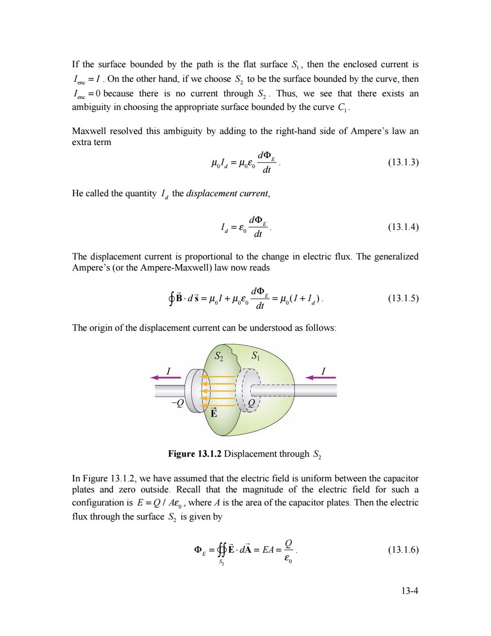
If the surface bounded by the path is the flat surface S,then the enclosed current is I=1.On the other hand,if we choose 2 to be the surface bounded by the curve,then =0 because there is no current through S2.Thus,we see that there exists an ambiguity in choosing the appropriate surface bounded by the curve C. Maxwell resolved this ambiguity by adding to the right-hand side of Ampere's law an extra term dΦE ola=odi (13.1.3) He called the quantity I the displacement current, d Ia=Eo dt (13.1.4) The displacement current is proportional to the change in electric flux.The generalized Ampere's (or the Ampere-Maxwell)law now reads ∮Bd5=/+4,e。 d=4,I+l) (13.1.5) The origin of the displacement current can be understood as follows: S2 Figure 13.1.2 Displacement through S2 In Figure 13.1.2,we have assumed that the electric field is uniform between the capacitor plates and zero outside.Recall that the magnitude of the electric field for such a configuration is E=/A,where A is the area of the capacitor plates.Then the electric flux through the surface S,is given by ΦE=∯EaA=EA=旦 (13.1.6) S2 13-4
13-4 If the surface bounded by the path is the flat surface 1 S , then the enclosed current is enc I = I . On the other hand, if we choose 2 S to be the surface bounded by the curve, then enc I = 0 because there is no current through 2 S . Thus, we see that there exists an ambiguity in choosing the appropriate surface bounded by the curve C1 . Maxwell resolved this ambiguity by adding to the right-hand side of Ampere’s law an extra term µ0 Id = µ0 ! 0 d"E dt . (13.1.3) He called the quantity Id the displacement current, Id = ! 0 d"E dt . (13.1.4) The displacement current is proportional to the change in electric flux. The generalized Ampere’s (or the Ampere-Maxwell) law now reads ! B! d ! s "" = µ0 I + µ0 # 0 d$E dt = µ0 (I + Id ) . (13.1.5) The origin of the displacement current can be understood as follows: Figure 13.1.2 Displacement through 2 S In Figure 13.1.2, we have assumed that the electric field is uniform between the capacitor plates and zero outside. Recall that the magnitude of the electric field for such a configuration is E = Q / A! 0 , where A is the area of the capacitor plates. Then the electric flux through the surface 2 S is given by !E = ! E" d ! A S2 "## = EA = Q $ 0 . (13.1.6)
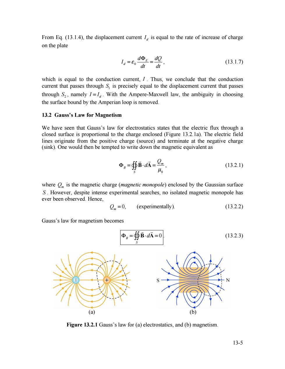
From Eq.(13.1.4),the displacement current I,is equal to the rate of increase of charge on the plate ,dΦE=d Ia=8o di di' (13.1.7) which is equal to the conduction current,I.Thus,we conclude that the conduction current that passes through S is precisely equal to the displacement current that passes through S2,namely I=1.With the Ampere-Maxwell law,the ambiguity in choosing the surface bound by the Amperian loop is removed. 13.2 Gauss's Law for Magnetism We have seen that Gauss's law for electrostatics states that the electric flux through a closed surface is proportional to the charge enclosed(Figure 13.2.1a).The electric field lines originate from the positive charge (source)and terminate at the negative charge (sink).One would then be tempted to write down the magnetic equivalent as Φ。=BadA= (13.2.1) where O is the magnetic charge (magnetic monopole)enclosed by the Gaussian surface S.However,despite intense experimental searches,no isolated magnetic monopole has ever been observed.Hence, Qm=0, (experimentally). (13.2.2) Gauss's law for magnetism becomes 中。=∯BdA=0 (13.2.3) (a) Figure 13.2.1 Gauss's law for (a)electrostatics,and (b)magnetism 13-5
13-5 From Eq. (13.1.4), the displacement current d I is equal to the rate of increase of charge on the plate 0 E d d dQ I dt dt ! " = = , (13.1.7) which is equal to the conduction current, I . Thus, we conclude that the conduction current that passes through 1 S is precisely equal to the displacement current that passes through 2 S , namely d I = I . With the Ampere-Maxwell law, the ambiguity in choosing the surface bound by the Amperian loop is removed. 13.2 Gauss’s Law for Magnetism We have seen that Gauss’s law for electrostatics states that the electric flux through a closed surface is proportional to the charge enclosed (Figure 13.2.1a). The electric field lines originate from the positive charge (source) and terminate at the negative charge (sink). One would then be tempted to write down the magnetic equivalent as !B = ! B"d ! A S "## = Qm µ0 , (13.2.1) where Qm is the magnetic charge (magnetic monopole) enclosed by the Gaussian surface S . However, despite intense experimental searches, no isolated magnetic monopole has ever been observed. Hence, Qm = 0, (experimentally). (13.2.2) Gauss’s law for magnetism becomes !B = ! B"d ! A S "## = 0 . (13.2.3) (a) (b) Figure 13.2.1 Gauss’s law for (a) electrostatics, and (b) magnetism