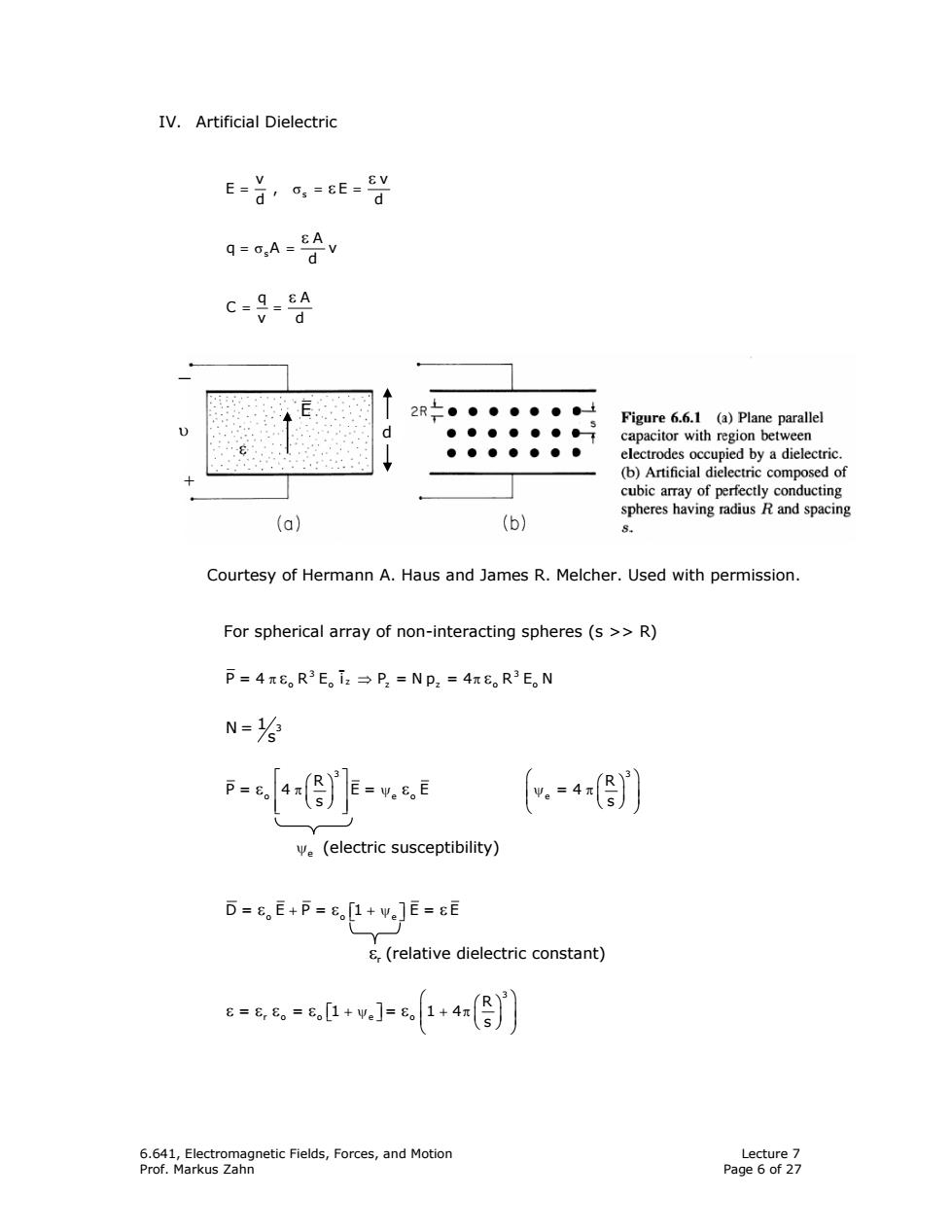
IV.Artificial Dielectric E V E-/G:-6ES d EA q=oA= d C=9=8A d 上● ●●●●●● Figure 6.6.1 (a)Plane parallel ●●●●●●● capacitor with region between ●●●●●● ● electrodes occupied by a dielectric. (b)Artificial dielectric composed of cubic array of perfectly conducting spheres having radius R and spacing (a) (b) Courtesy of Hermann A.Haus and James R.Melcher.Used with permission. For spherical array of non-interacting spheres(s >R) p=4元8。R3E。i2→P2=Np2=4πE。R3E。N N=⅓ p=0 4π R s =y。8。E e(electric susceptibility) D=8E+P=8o[1+Ve]E=8E 8(relative dielectric constant) 8=8,6=6,1+v]=1+4(餐) 6.641,Electromagnetic Fields,Forces,and Motion Lecture 7 Prof.Markus Zahn Page 6 of 27
6.641, Electromagnetic Fields, Forces, and Motion Lecture 7 Prof. Markus Zahn Page 6 of 27 IV. Artificial Dielectric s v v E, E d d = σ= = ε ε s A qA v d =σ = ε = = q Aε C v d Courtesy of Hermann A. Haus and James R. Melcher. Used with permission. For spherical array of non-interacting spheres (s >> R) π⇒ π ε ε _ 3 3 z P = 4 R E i P = N p = 4 R E N oo z z oo N = 1 3 s ⎡⎤ ⎛ ⎞ ⎛⎞ ⎛⎞ ⎢ ⎥ π ψ ψπ ⎜ ⎟ ⎜⎟ ⎜⎟ ⎢ ⎥ ⎝⎠ ⎝⎠ ⎣⎦ ⎝ ⎠ ε ε 3 3 o eo e R R P= 4 E= E =4 s s ψe (electric susceptibility) + +ψ ⎡ ⎤ ⎣ ⎦ εε ε D= E P= 1 E= E o oe r ε (relative dielectric constant) ⎛ ⎞ ⎛ ⎞ ⎡ ⎤ +ψ + π ⎜ ⎟ ⎣ ⎦ ⎜ ⎟ ⎝ ⎠ ⎝ ⎠ ε εε ε ε 3 ro o e o R = = 1 = 14 s _ d + ε E υ
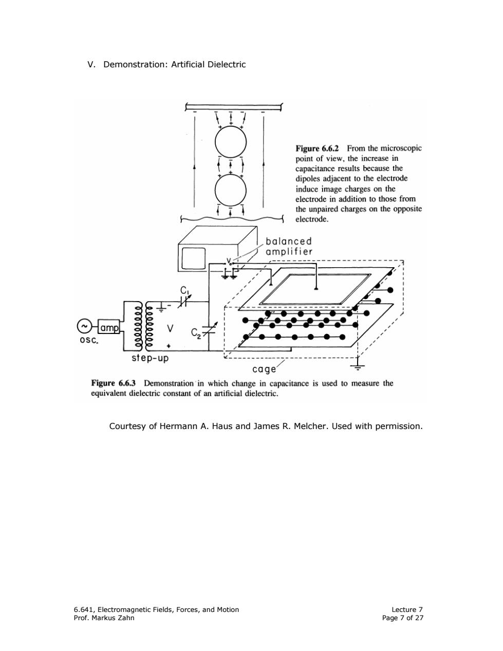
V.Demonstration:Artificial Dielectric Figure 6.6.2 From the microscopic point of view,the increase in capacitance results because the dipoles adjacent to the electrode induce image charges on the electrode in addition to those from the unpaired charges on the opposite electrode. balanced amplifier 心amp osc. 25555. step-up cage Figure 6.6.3 Demonstration'in which change in capacitance is used to measure the equivalent dielectric constant of an artificial dielectric. Courtesy of Hermann A.Haus and James R.Melcher.Used with permission. 6.641,Electromagnetic Fields,Forces,and Motion Lecture 7 Prof.Markus Zahn Page 7 of 27
6.641, Electromagnetic Fields, Forces, and Motion Lecture 7 Prof. Markus Zahn Page 7 of 27 V. Demonstration: Artificial Dielectric Courtesy of Hermann A. Haus and James R. Melcher. Used with permission
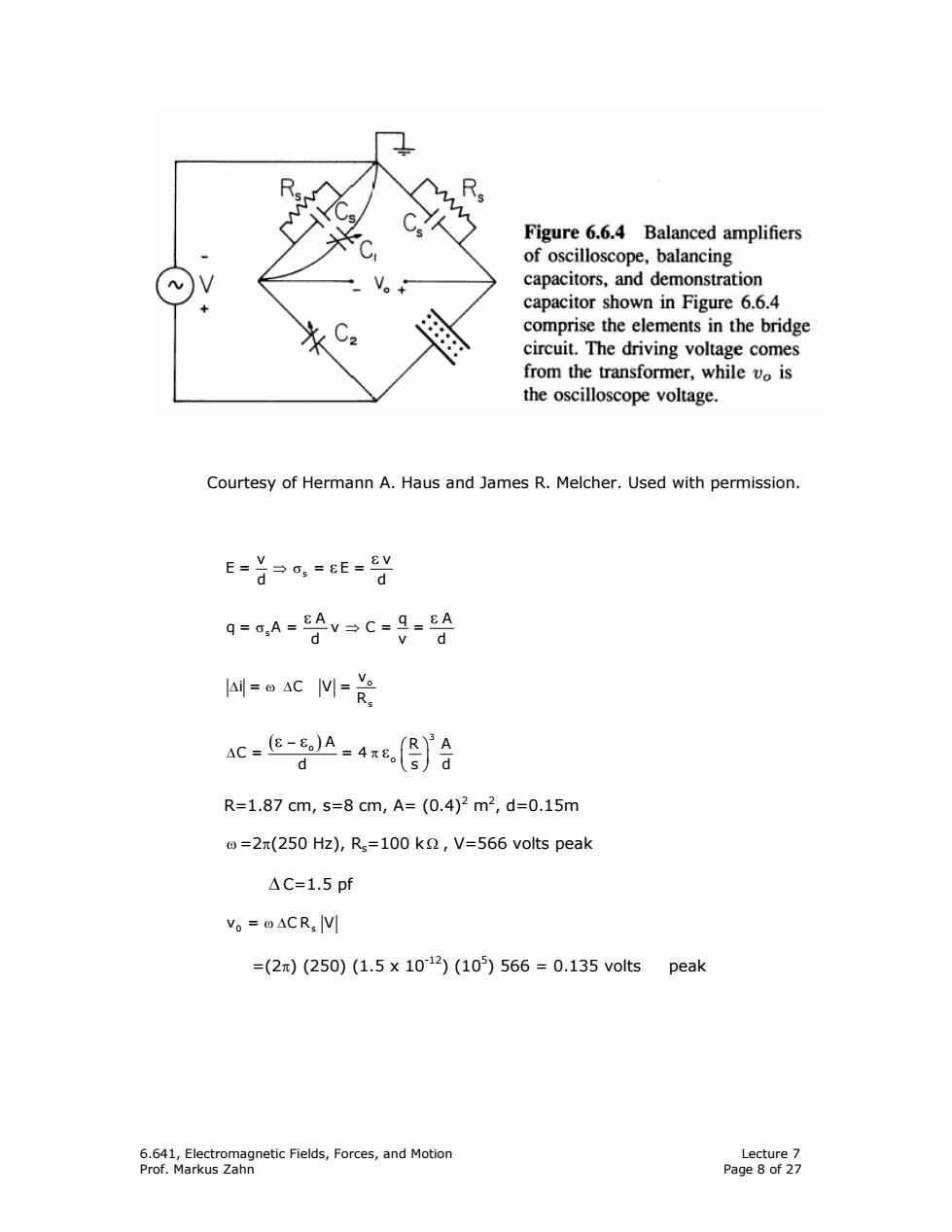
Figure 6.6.4 Balanced amplifiers of oscilloscope,balancing capacitors,and demonstration capacitor shown in Figure 6.6.4 8 comprise the elements in the bridge circuit.The driving voltage comes from the transformer,while vo is the oscilloscope voltage. Courtesy of Hermann A.Haus and James R.Melcher.Used with permission. E=首p,=eE=y d q=o,A=8Av→C=9=8A d d AC M sc.e-g.4合 d R=1.87cm,s=8cm,A=(0.4)2m2,d=0.15m @=2(250 Hz),Rs=100 k,V=566 volts peak △C=1.5pf V。=oACR,V =(2π)(250)(1.5×10¹²)(105)566=0.135 volts peak 6.641,Electromagnetic Fields,Forces,and Motion Lecture 7 Prof.Markus Zahn Page 8 of 27
6.641, Electromagnetic Fields, Forces, and Motion Lecture 7 Prof. Markus Zahn Page 8 of 27 Courtesy of Hermann A. Haus and James R. Melcher. Used with permission. s v v E= = E= d d ⇒ σ ε ε s A qA q= A= v C= = d vd σ ⇒ ε ε ∆ ω∆ o s v i= C V= R ( − ) ⎛ ⎞ ∆ π ⎜ ⎟ ⎝ ⎠ ε ε ε 3 o o A R A C= =4 d sd R=1.87 cm, s=8 cm, A= (0.4)2 m2 , d=0.15m ω =2π(250 Hz), Rs=100 k Ω , V=566 volts peak ∆ C=1.5 pf v = CR V 0 s ω ∆ =(2π) (250) (1.5 x 10⁻¹²) (105 ) 566 = 0.135 volts peak

VI.Plasma Conduction Model(Classical) m0=aE-mv文-R n m昨=-qE-mvV-p dt n p.=n.kT,p.=n_kT k=1.38 x 10²³ joules/K Boltzmann Constant A.London Model of Superconductivity[T→O,v±→O] m..m. dt =-q.E dv- j.q.n,v,J=-q.n.v. 0-品an)=ang-ana目-E m.m 0+e 票-是an)qn祭-qng周-E m.m 06_8 @.=an,of.-92n (plasma frequency) m.E m 8 For electrons:q-=1.6 x 10¹⁹ Coulombs,m.=9.1 x 1031 kg n.=1020/m3,e=8。÷8.854x10-12 farads/,m 0p.=1 g2n≈5.6x101rad/s m.8 =2 g=≈9x100Hz 6.641,Electromagnetic Fields,Forces,and Motion Lecture 7 Prof.Markus Zahn Page 9 of 27
6.641, Electromagnetic Fields, Forces, and Motion Lecture 7 Prof. Markus Zahn Page 9 of 27 VI. Plasma Conduction Model (Classical) + + + + ++ + + ∇ −ν − dv p m =q E m v dt n − − − − −− − − ∇ − −ν − dv p m = qE m v dt n p = n kT , p = n kT ++ −− k=1.38 x 10⁻²³ joules/o K Boltzmann Constant A. London Model of Superconductivity [ T → ν→ 0, 0 ± ] dv dv m =qE , m = qE dt dt + − ++− − − + − + − ++ −− J =q n v , J = qnv − ( ) ( ) q E 2 dJ d dv q n q n v =q n =q n = E dt dt dt m m + + + + + ++ ++ ++ + + + = ω + ε 2 p ( ) ( ) q E 2 dJ d dv q n = qnv = qn = qn = E dt dt dt m m − − − − − −− −− −− − − − − − −− ε 2 + + − − + − + − ω ω ε ε 2 2 2 2 p p q n q n = ,= m m (ωp = plasma frequency) For electrons: q-=1.6 x 10⁻¹⁹ Coulombs, m-=9.1 x 10⁻³¹ kg n-=1020/m3 , 12 o 8.854 x 10− ε = ≈ ε farads/m − − − − ω ≈ ε 2 11 p q n = 5.6 x 10 m rad/s − − ≈ π ωp 10 pf = 9 x10 2 Hz − ωp