This implies that the number of magnetic field lines entering a closed surface is equal to the number of field lines leaving that surface.There is no magnetic source or sink.In addition,the lines must be continuous with no starting or end points.In fact,as shown in Figure 13.2.1(b)for a bar magnet,the field lines that emanate from the north pole to the south pole outside the magnet return within the magnet and form closed loops. 13.3 Maxwell's Equations We now have four equations that form the foundation of electromagnetic phenomena: Law Equation Physical Interpretation Gauss's law for E ∯E.A= Electric flux through a closed surface Eo is proportional to the charge enclosed Faraday's law ∮Ed5=-Φ2 Changing magnetic flux is associated with an electric field Gauss's law for B ∯B=0 The total magnetic flux through a closed surface is zero Ampere-Maxwell law dΦE fB.ds=1+4e。di Electric current and changing electric flux is associated with a magnetic field Collectively they are known as Maxwell's Equations.The above equations may also be written in differential form as V.E=P Eo P×E=-那 (13.3.1) 7.B=0, V×B=4,J+ea where p and J are the free charge and the conduction current densities,respectively. In the absence of charged sources,O=0 and I=0,the above integral equations become 13-6
13-6 This implies that the number of magnetic field lines entering a closed surface is equal to the number of field lines leaving that surface. There is no magnetic source or sink. In addition, the lines must be continuous with no starting or end points. In fact, as shown in Figure 13.2.1(b) for a bar magnet, the field lines that emanate from the north pole to the south pole outside the magnet return within the magnet and form closed loops. 13.3 Maxwell’s Equations We now have four equations that form the foundation of electromagnetic phenomena: Law Equation Physical Interpretation Gauss's law for E ! ! E! d ! A S """ = Q # 0 Electric flux through a closed surface is proportional to the charge enclosed Faraday's law ! E! d ! s = " d#B dt "$ Changing magnetic flux is associated with an electric field Gauss's law for B ! ! B! d ! A S """ = 0 The total magnetic flux through a closed surface is zero Ampere ! Maxwell law ! B! d ! s = µ0 I + µ0 " 0 d#E dt "$ Electric current and changing electric flux is associated with a magnetic field Collectively they are known as Maxwell’s Equations. The above equations may also be written in differential form as ! " ! E = # $ 0 , ! % ! E = & ' ! B 't , ! " ! B = 0, ! % ! B = µ0 ! J + µ0 $ 0 ' ! E 't . (13.3.1) where ! and J ! are the free charge and the conduction current densities, respectively. In the absence of charged sources, Q = 0 and I = 0 , the above integral equations become
∯EdA=0, ∮2ds= dΦB dt (13.3.2) ∯B.dA=0, dΦE ∮B-ds=4edh An important consequence of Maxwell's equations,as we shall see below,is the prediction of the existence of electromagnetic waves that travel with the speed of light c=1/.The reason is due to the fact that a changing electric field is associated with a magnetic field and vice versa,and the coupling between the two fields leads to the generation of electromagnetic waves.In 1887,H.Hertz confirmed this prediction. 13.4 Plane Traveling Electromagnetic Waves To examine the properties of the electromagnetic waves,let's consider an electromagnetic wave propagating in the +x-direction,with a uniform electric field E pointing in the +y-direction and a uniform magnetic field B in the +z-direction.At any instant both E and B are uniform over any yz-plane perpendicular to the direction of propagation.This means that for any value of x,the electric and magnetic fields are the same at all points yz-plane perpendicular to that value ofx.The electric and magnetic field are independent of the (y,z)coordinates.Therefore the electric and magnetic fields are only functions of the (x,t)coordinates,E(x,t)=E (x,t)j and B(x,t)=B.(x,t)k E(0,0) E(x,ct) E(x2,ct2) B(0,0) B(x.cl) B(x,,ct) Figure 13.4.1 Electric and magnetic fields at a few selected points along the x-axis associated with a plane electromagnetic wave. 13-7
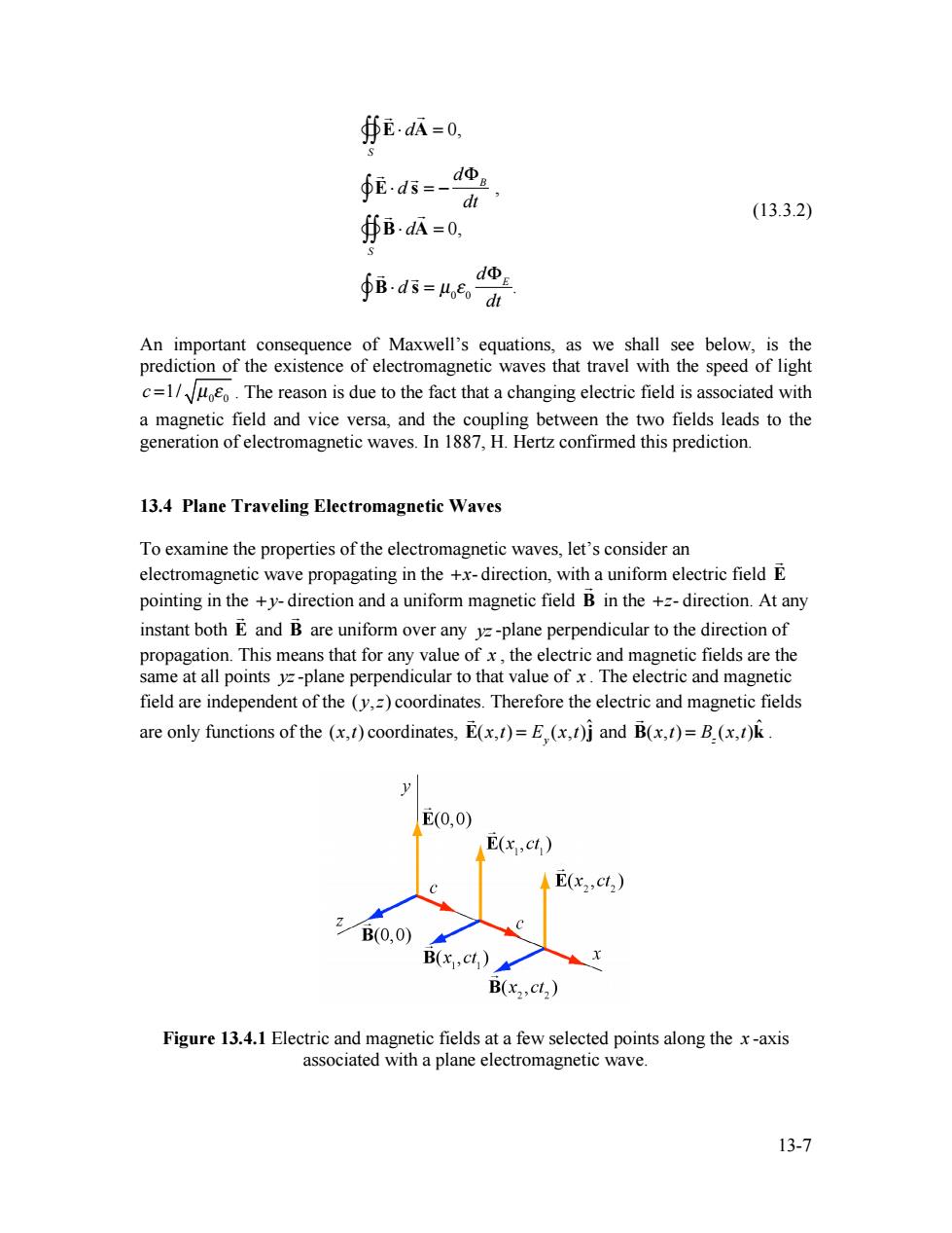
13-7 ! E! d ! A S """ = 0, ! E! d ! s = # d$B dt #" , ! B! d ! A S """ = 0, ! B! d ! s = µ0 % 0 d$E dt #" . (13.3.2) An important consequence of Maxwell’s equations, as we shall see below, is the prediction of the existence of electromagnetic waves that travel with the speed of light 0 0 c =1/ µ ! . The reason is due to the fact that a changing electric field is associated with a magnetic field and vice versa, and the coupling between the two fields leads to the generation of electromagnetic waves. In 1887, H. Hertz confirmed this prediction. 13.4 Plane Traveling Electromagnetic Waves To examine the properties of the electromagnetic waves, let’s consider an electromagnetic wave propagating in the +x- direction, with a uniform electric field E ! pointing in the + y- direction and a uniform magnetic field B ! in the +z- direction. At any instant both E ! and B ! are uniform over any yz-plane perpendicular to the direction of propagation. This means that for any value of x , the electric and magnetic fields are the same at all points yz-plane perpendicular to that value of x . The electric and magnetic field are independent of the ( y,z) coordinates. Therefore the electric and magnetic fields are only functions of the (x,t) coordinates, ! E(x,t) = E y (x,t)ˆ j and ! B(x,t) = Bz (x,t)kˆ . Figure 13.4.1 Electric and magnetic fields at a few selected points along the x -axis associated with a plane electromagnetic wave
In the representation shown in Figure 13.4.1,at time=0,consider the vectors E(0,0) and B(0,0),corresponding to the electric and magnetic fields on the plane x=0.We show two additional pairs of electric and magnetic vectors representing E(x)and B(xc on the plane x=c,and E(x2,ct2)and B(x2ct)on the plane x2=cl2 This (non-physical)electric and magnetic field is called a plane wave because at any instant both E and B are uniform over any plane perpendicular to the direction of propagation.In addition,the wave is transverse because both fields are perpendicular to the direction of propagation,which points in the direction of the cross product Ex B Using Maxwell's equations,we may obtain the relationship between the magnitudes of the fields and their derivatives.To see this,consider a rectangular loop that lies in the xy-plane,with the left side of the loop at x and the right at x+Ar.The bottom side of the loop is located at y and the top of the loop is located at y+Ay as shown in Figure 13.4.2.Let the unit vector normal to the loop be in the positive =-direction,n=k E(x) E(x+△x) B Figure 13.4.2 Spatial variation of the electric field E Recall Faraday's law 6=-BA (13.4.1) In order to evaluate the left-hand-side of Eq.(13.4.1),we integrate counterclockwise around the closed path shown in Figure 13.4.2, ∮E·s=E,(x+Ax)4y-E,x)Ay (13.4.2) We can use the Taylor expansion to approximate 13-8
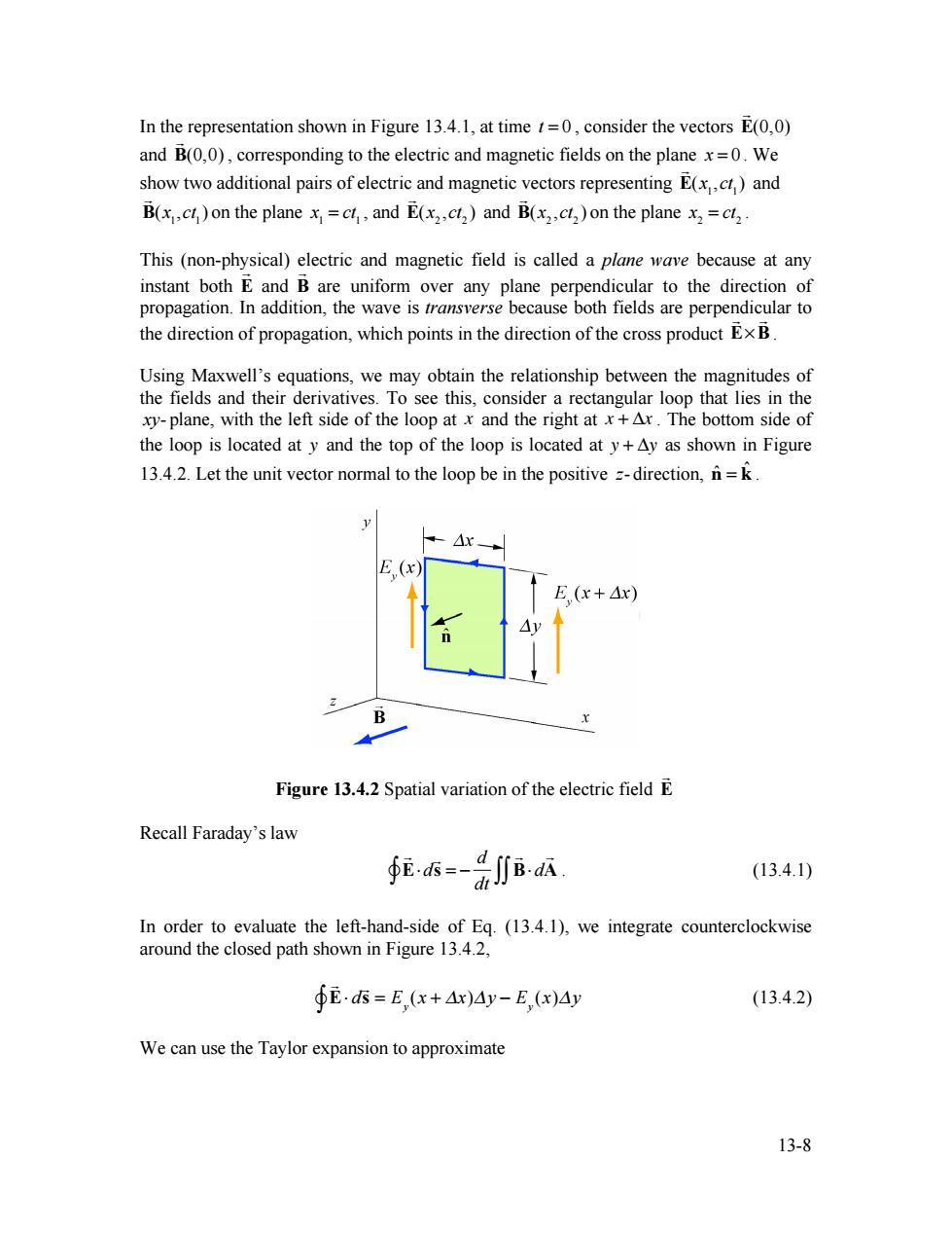
13-8 In the representation shown in Figure 13.4.1, at time t = 0 , consider the vectors ! E(0,0) and ! B(0,0) , corresponding to the electric and magnetic fields on the plane x = 0 . We show two additional pairs of electric and magnetic vectors representing ! E(x1,ct 1) and ! B(x1,ct 1) on the plane x1 = ct 1 , and ! E(x2 ,ct 2 ) and ! B(x2 ,ct 2 ) on the plane x2 = ct 2 . This (non-physical) electric and magnetic field is called a plane wave because at any instant both E ! and B ! are uniform over any plane perpendicular to the direction of propagation. In addition, the wave is transverse because both fields are perpendicular to the direction of propagation, which points in the direction of the cross product E!B ! ! . Using Maxwell’s equations, we may obtain the relationship between the magnitudes of the fields and their derivatives. To see this, consider a rectangular loop that lies in the xy- plane, with the left side of the loop at x and the right at x + !x . The bottom side of the loop is located at y and the top of the loop is located at y + !y as shown in Figure 13.4.2. Let the unit vector normal to the loop be in the positive z- direction, nˆ = kˆ . Figure 13.4.2 Spatial variation of the electric field E ! Recall Faraday’s law ! E!d ! s = " d dt ! B! d ! "# ## A . (13.4.1) In order to evaluate the left-hand-side of Eq. (13.4.1), we integrate counterclockwise around the closed path shown in Figure 13.4.2, ! E! d ! s "" = E y (x + #x)#y $ E y (x)#y (13.4.2) We can use the Taylor expansion to approximate
aEAx+… E.(x+Ax)=E,(x)+x (13.4.3) Then left-hand-side of Faraday's law becomes ∮Es= E2△xAy (13.4.4) Ox We assume that Ar and Ay are very small such that the time derivative of the = component of the magnetic field is nearly uniform over the area element.Then the rate of change of magnetic flux on the right-hand-side of Eq.(13.4.1)is given by s=- B△x△y, (13.4.5) Equating the two sides of Faraday's Law and dividing through by the area AxAy yields (13.4.6) Eq.(13.4.6)result indicates that at each point in space a time-varying magnetic field is associated with a spatially varying electric field. The second condition on the relationship between the electric and magnetic fields may be deduced by using the Ampere-Maxwell equation: B西=4气Ea (13.4.7) Consider a rectangular loop in the xy-plane depicted in Figure 13.4.3,with a unit normal n=j. E,(x) B.(x) △X 42 B(x+△x) Figure 13.4.3 Spatial variation of the magnetic field B 13-9
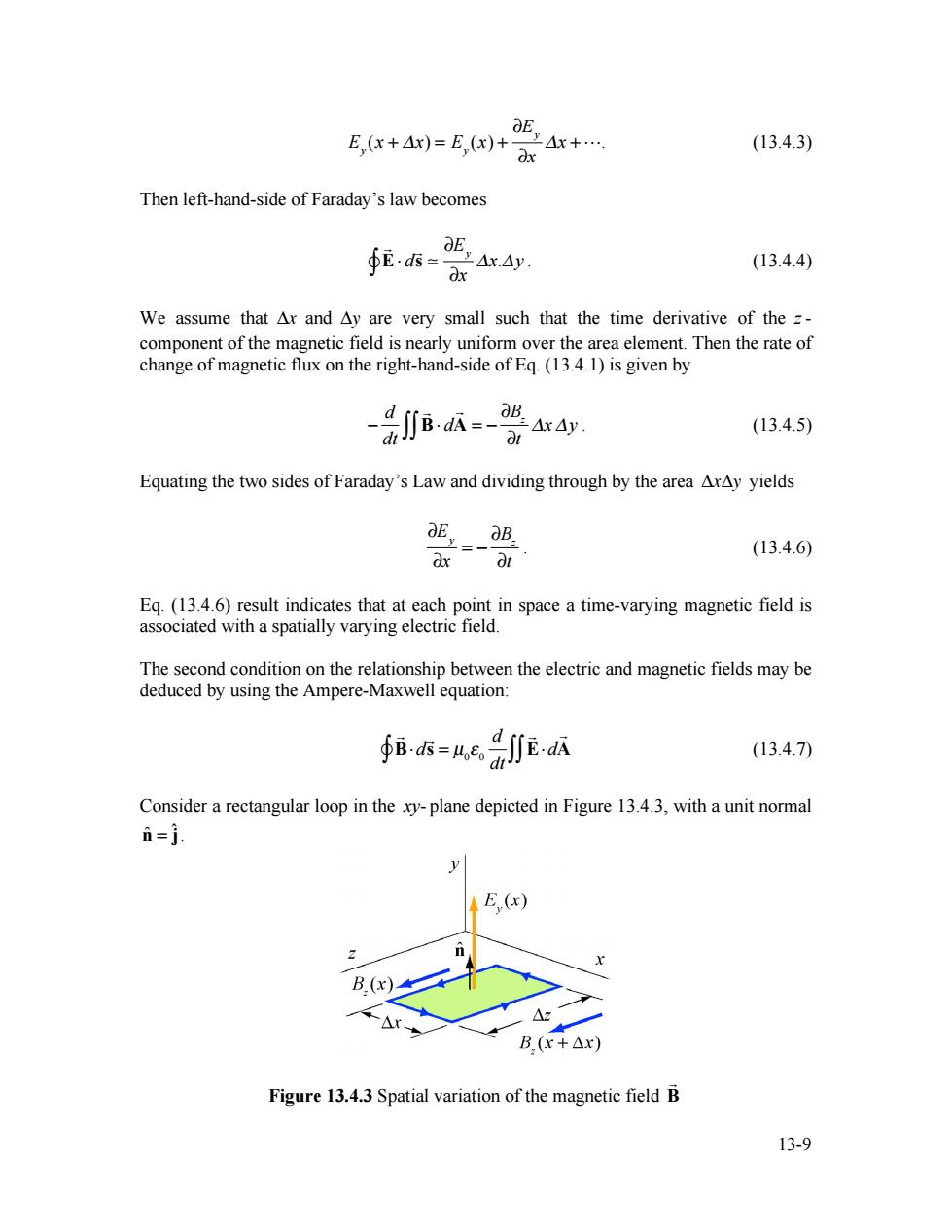
13-9 E y (x + !x) = E y (x) + "E y "x !x +!. (13.4.3) Then left-hand-side of Faraday’s law becomes ! E! d ! s "" # #E y #x $x.$y . (13.4.4) We assume that !x and !y are very small such that the time derivative of the z - component of the magnetic field is nearly uniform over the area element. Then the rate of change of magnetic flux on the right-hand-side of Eq. (13.4.1) is given by ! d dt ! B" d ! ## A = ! $Bz $t %x %y . (13.4.5) Equating the two sides of Faraday’s Law and dividing through by the area !x!y yields !E y !x = " !Bz !t . (13.4.6) Eq. (13.4.6) result indicates that at each point in space a time-varying magnetic field is associated with a spatially varying electric field. The second condition on the relationship between the electric and magnetic fields may be deduced by using the Ampere-Maxwell equation: ! B!d ! s = µ0 " 0 d dt "# ! E!d ! ## A (13.4.7) Consider a rectangular loop in the xy- plane depicted in Figure 13.4.3, with a unit normal ˆ nˆ = j. Figure 13.4.3 Spatial variation of the magnetic field B !
We begin by evaluating the line integral of the magnetic field counterclockwise around the closed path shown in Figure 13.4.3, ∮B-ds=B.(x)Az-B(+△x)A:. (13.4.8) We now use the Taylor expansion to approximate a B.(x+Ax)=B.(x)+ 三△x+… (13.4.9) O Then left-hand-side of the Maxwell-Ampere law then becomes 6B.d3=-O8 △x△z」 (13.4.10) dx We assume that Ax and Az are very small such that the time derivative of the y- component of the electric field is nearly uniform over the area element.Then the rate of change of electric flux on the right-hand-side of Eq.(13.4.7)is given by .AxAz. A品E-=e (13.4.11) Equating the two sides of the Maxwell-Ampere law and dividing by AxAz yields B.=Ho t E V (13.4.12) Ox Eq.(13.4.12)result indicates that at each point in space a time-varying electric field is associated by a spatially varying magnetic field. Egs.(13.4.6)and(13.4.12)are coupled differential equations.To uncouple them,we first take another partial derivative of Eq.(13.4.6)with respect to x, a=arar arl ax a∂B (13.4.13) We have assumed that the field B is sufficiently well behaved such that the partial derivatives are interchangeable, 13-10
13-10 We begin by evaluating the line integral of the magnetic field counterclockwise around the closed path shown in Figure 13.4.3, ! B! d ! s "" = Bz (x)#z $ Bz (x + #x)#z . (13.4.8) We now use the Taylor expansion to approximate Bz (x + !x) = Bz (x) + "Bz "x !x +!. (13.4.9) Then left-hand-side of the Maxwell-Ampere law then becomes ! B! d ! s "" = # $Bz $x %x%z. (13.4.10) We assume that !x and !z are very small such that the time derivative of the y - component of the electric field is nearly uniform over the area element. Then the rate of change of electric flux on the right-hand-side of Eq. (13.4.7) is given by µ0 ! 0 d dt ! E" d ! ## A = µ0 ! 0 $E y $t %x %z . (13.4.11) Equating the two sides of the Maxwell-Ampere law and dividing by !x!z yields ! "Bz "x = µ0 # 0 "E y "t . (13.4.12) Eq. (13.4.12) result indicates that at each point in space a time-varying electric field is associated by a spatially varying magnetic field. Eqs. (13.4.6) and (13.4.12) are coupled differential equations. To uncouple them, we first take another partial derivative of Eq. (13.4.6) with respect to x, !2 E y !x 2 = " ! !x !Bz !t # $ % & ' ( = " ! !t !Bz !x # $ % & ' ( (13.4.13) We have assumed that the field Bz is sufficiently well behaved such that the partial derivatives are interchangeable