roots, B(s)R(1)R(2) R(n) .+ +KS) A(S)s-P1)s-P(2) s-P(n) Vectors B and A specify the coefficients of the numerator and denominator polynomials in descending powers ofs.The residues are returned in the column vector R,the pole locations in column vector P,and the direct terms in row vector K.The number of poles is n=length(A)-1 =length(R)= length(P).The direct term coefficient vector is empty if length(B)<length(A), otherwise length(K)=length(B)-length(A)+1. If P(j)=.=P(j+m-1)is a pole of multplicity m,then the expansion includes terms of the form R(j)R(j+1) R(j+m-1) s-P(j)(s-P(j))2 (s-P(j))m [B,A]=RESIDUE(R,P,K),with 3 input arguments and 2 output arguments,converts the partial fraction expansion back to the polynomials with coefficients in Band A. 例3:对(3x+2x3+5x2+4x+6)/(x5+3x4+4x3+2x2+7x+2)做部分分式展 公 a=134272 b-32546: [rs,k]=residue(b,a) r= 1.1274+1.1513i 1.1274-1.1513i -0.0232-0.0722i -0.0232+0.0722 0.7916 s=
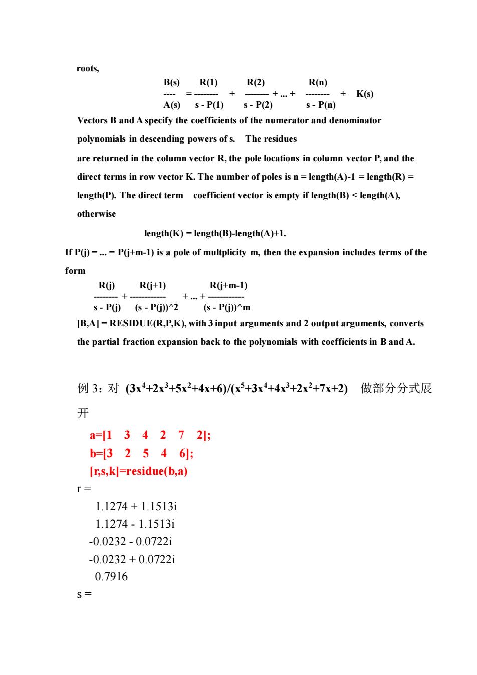
roots, B(s) R(1) R(2) R(n) - = - + - + . + - + K(s) A(s) s - P(1) s - P(2) s - P(n) Vectors B and A specify the coefficients of the numerator and denominator polynomials in descending powers of s. The residues are returned in the column vector R, the pole locations in column vector P, and the direct terms in row vector K. The number of poles is n = length(A)-1 = length(R) = length(P). The direct term coefficient vector is empty if length(B) < length(A), otherwise length(K) = length(B)-length(A)+1. If P(j) = . = P(j+m-1) is a pole of multplicity m, then the expansion includes terms of the form R(j) R(j+1) R(j+m-1) - + - + . + - s - P(j) (s - P(j))^2 (s - P(j))^m [B,A] = RESIDUE(R,P,K), with 3 input arguments and 2 output arguments, converts the partial fraction expansion back to the polynomials with coefficients in B and A. 例 3:对 (3x4+2x3+5x2+4x+6)/(x5+3x4+4x3+2x2+7x+2) 做部分分式展 开 a=[1 3 4 2 7 2]; b=[3 2 5 4 6]; [r,s,k]=residue(b,a) r = 1.1274 + 1.1513i 1.1274 - 1.1513i -0.0232 - 0.0722i -0.0232 + 0.0722i 0.7916 s =

-1.7680+1.2673i -1.7680-1.2673i 0.4176+1.11301 0.4176-1.1130i -0.2991 k= 川(分母阶数高于分子阶数时,k将是空矩阵,表示无此项) 例5:对一组实验数据进行多项式最小二乘拟合(least square fit)) x=12345: %实验数据 y-5.543.1128290.7498.4h; p=polyfit(x,y,3) %做三阶多项式拟合 x2=1:.1:5; y2=polyval(p,x2); %根据给定值计算多项式结果 plot(x,y,'o',x2,y2) 一.线性代数(Linear Algebra) 解线性方程(Linear equation)就是找出是否存在一个唯一的矩阵x,使 得a,b满足关系: ax=b或xa=b MALAB中x=ab是方程ax=b的解,x=b/a是方程式xa=b的解。 通常线性方程多写成ax=b,“1”较多用,两者的关系为: (b/a'=(a\b) 系数矩阵a可能是m行n列的,有三种情况: 方阵系统:(Square matrix)m=n可求出精确解(a必须是非奇异 (nonsingular),即满秩(full rank)) *超定系统:(Overdetermind system)m>n可求出最小二乘解 *欠定系统:(Underdetermind system)m<知可尝试找出含有最少m个基 解或最小范数解 MATLAB对不同形式的参数矩阵,采用不同的运算法则来处理,它会 自动检测参数矩阵,以区别下面几种形式:
-1.7680 + 1.2673i -1.7680 - 1.2673i 0.4176 + 1.1130i 0.4176 - 1.1130i -0.2991 k = [] (分母阶数高于分子阶数时,k 将是空矩阵,表示无此项) 例 5:对一组实验数据进行多项式最小二乘拟合(least square fit) x=[1 2 3 4 5]; % 实验数据 y=[5.5 43.1 128 290.7 498.4]; p=polyfit(x,y,3) %做三阶多项式拟合 x2=1:.1:5; y2=polyval(p,x2); % 根据给定值计算多项式结果 plot(x,y,’o’,x2,y2) 一. 线性代数(Linear Algebra) 解线性方程(Linear equation)就是找出是否存在一个唯一的矩阵 x,使 得 a,b 满足关系: ax=b 或 xa=b MALAB 中 x=a\b 是方程 ax=b 的解, x=b/a 是方程式 xa=b 的解。 通常线性方程多写成 ax=b,“\”较多用,两者的关系为: (b/a)’=(a’\b’) 系数矩阵 a 可能是 m 行 n 列的,有三种情况: *方阵系统: (Square matrix) m=n 可求出精确解(a 必须是非奇异 (nonsingular),即满秩(full rank)) *超定系统:(Overdetermind system)m>n 可求出最小二乘解 *欠定系统:(Underdetermind system) m<n 可尝试找出含有最少 m 个基 解或最小范数解 MATLAB 对不同形式的参数矩阵,采用不同的运算法则来处理,它会 自动检测参数矩阵,以区别下面几种形式:

*三角矩阵(Triangular Matri) *对称正定矩阵(symmetrical positive determined matrix) *非奇异方阵(Nonsingular matrix) *超定系统(Overdetermind system) *欠定系统(Underdetermind system) L.方阵系统:(Square array) 最常见的是系数矩阵为方阵a,常数项b为列矢量,其解x可写成x=ab, x和b大小相同。 例1:求方阵系统的根。 a=16755139:17181 b=16134 x=alb a= 11 6 5 13 9 17 1 b= 16 13 4 X= 3.9763 5.4455 -8.6303 例2:假如a,b为两个大小相同的矩阵,求方阵系统的根。 a=459;18195;14131 b=1512;31519;7610 x=alb C=a*x
*三角矩阵(Triangular Matrix) *对称正定矩阵(symmetrical positive determined matrix) *非奇异方阵(Nonsingular matrix) *超定系统(Overdetermind system) *欠定系统(Underdetermind system) 1. 方阵系统:(Square array) 最常见的是系数矩阵为方阵a,常数项b为列矢量, 其解x可写成x=a\b, x 和 b 大小相同。 例 1: 求方阵系统的根。 a=[11 6 7; 5 13 9; 17 1 8] b=[16 13 4]’ x=a\b a = 11 6 7 5 13 9 17 1 8 b = 16 13 4 x = 3.9763 5.4455 -8.6303 例 2:假如 a,b 为两个大小相同的矩阵,求方阵系统的根。 a=[4 5 9; 18 19 5; 1 4 13] b=[1 5 12; 3 15 19; 7 6 10] x=a\b C=a*x

as 4 5 9 1819 5 1 4 13 b= 1 12 3 15 19 610 X= -3.6750 -0.7333 2.9708 37250 1.4667 -2.1292 -0.3250 0.0667 1.1958 C= 1.00005.000012.0000 3.0000 15.0000 19.0000 7.00006.000010.0000 若方阵a的各个行矢量线性相关((linear correlation),则称方阵a为奇异矩阵。 这时线性方程将有无穷多组解。若方阵是奇异矩阵,则反斜线运算因子将发出 警告信息。 2.超定系统(Overdetermind system) 实验数据较多,寻求他们的曲线拟合。 如在t内测得一组数据y: t y
a = 4 5 9 18 19 5 1 4 13 b = 1 5 12 3 15 19 7 6 10 x = -3.6750 -0.7333 2.9708 3.7250 1.4667 -2.1292 -0.3250 0.0667 1.1958 C = 1.0000 5.0000 12.0000 3.0000 15.0000 19.0000 7.0000 6.0000 10.0000 若方阵a 的各个行矢量线性相关(linear correlation),则称方阵a 为奇异矩阵。 这时线性方程将有无穷多组解。若方阵是奇异矩阵,则反斜线运算因子将发出 警告信息。 2.超定系统(Overdetermind system) 实验数据较多,寻求他们的曲线拟合。 如在 t 内测得一组数据 y: t y

0.0 0.82 0.3 0.72 0.8 0.63 1.1 0.60 1.6 0.55 2.2 0.50 这些数据显然有衰减指数趋势:y(t)c1+e2e 此方程意为y矢量可以由两个矢量逐步逼近而得,一个是单行的常数 矢量,一个是由指数et项构成,两个参数c1和c2可用最小二乘法求得,它 们表示实验数据与方程y(t)c1+c2e之间距离的最小平方和。 例1:求上述数据的最小二乘解。将数据带入方程式y)C1+2et中,可 得到含有两个未知数的6个等式,可写成6行2列的矩阵e. 00.30.81.11.62.2; y=0.820.720.630.600.550.50; e=[ones(size(t))exp(-t)] %求6个y()方程的系数矩阵 c=ely %求方程的解 e= 1.0000 1.0000 1.0000 0.7408 1.0000 0.4493 1.0000 0.3329 1.0000 0.2019 1.0000 0.1108 c= 0.4744 0.3434 带入方程得:y(t)0.4744+0.3434et 用此方程可绘制曲线: t=00.30.81.11.62.2'; y0.820.720.630.600.550.50: tl=0:0.1:2.5]';yl=lones(size(tI)),exp(-tI)]*c
0.0 0.82 0.3 0.72 0.8 0.63 1.1 0.60 1.6 0.55 2.2 0.50 这些数据显然有衰减指数趋势: y(t)~c1+c2e -t 此方程意为 y 矢量可以由两个矢量逐步逼近而得,一个是单行的常数 矢量,一个是由指数 e -t项构成,两个参数 c1 和 c2 可用最小二乘法求得,它 们表示实验数据与方程 y(t)~c1+c2e -t之间距离的最小平方和。 例 1: 求上述数据的最小二乘解。将数据带入方程式 y(t)~c1+c2e -t 中,可 得到含有两个未知数的 6 个等式,可写成 6 行 2 列的矩阵 e. t=[0 0.3 0.8 1.1 1.6 2.2]’; y=[0.82 0.72 0.63 0.60 0.55 0.50]’; e=[ones(size(t)) exp(-t)] %求 6 个 y(t)方程的系数矩阵 c=e\y % 求方程的解 e = 1.0000 1.0000 1.0000 0.7408 1.0000 0.4493 1.0000 0.3329 1.0000 0.2019 1.0000 0.1108 c = 0.4744 0.3434 带入方程得:y(t)~0.4744+0.3434e-t 用此方程可绘制曲线: t=[0 0.3 0.8 1.1 1.6 2.2]’; y=[0.82 0.72 0.63 0.60 0.55 0.50]’; t1=[0:0.1:2.5]’; y1=[ones(size(t1)),exp(-t1)]*c