实验二连续时间信号的运算 一、实验目的 1、掌握连续时间信号时域运算的MATLAB实现方法。 2、掌握MATLAB内部函数的应用。 二、实验原理 信号的基本运算包括信号的相加(减)和相乘(除)。信号的时域变换包括信号的平移、 翻转、反折以及尺度变换、微分、积分等。 1、时移:f)→f(u±) 2、反折:f(t→f(-) 3、尺度变换:f(t)→f(a),a>1,信号压缩:a<1,信号扩展: 4、信号的微分:f0→0 5、信号的积分:f)→frr 6、信号的相加:f)=f()+f5() 7、信号的相乘:f)=()*f5() 三、实验内容 1、信号的移位、反稻、尺度变换 【例2-1】已知信号如图2-1所示,试绘出f1+2)、 f(t) f(-)、f21)的波形图。 可以在MATLAB的work目录下先创建原信号f() 函数fctm,程序如下: function f=fct(t) f=(u(t+2)-u(t)+(-t+1).*(u(t)-u(t-1)): 在程序中调用上述函数来绘制所要求的信号波形, 图2-1f()信号
实验二 连续时间信号的运算 一、实验目的 1、掌握连续时间信号时域运算的 MATLAB 实现方法。 2、掌握 MATLAB 内部函数的应用。 二、实验原理 信号的基本运算包括信号的相加(减)和相乘(除)。信号的时域变换包括信号的平移、 翻转、反折以及尺度变换、微分、积分等。 1、时移: ( ) ( ) 0 f t f t t 2、反折: f (t) f (t) 3、尺度变换: f (t) f (at) , a 1 ,信号压缩; a 1 ,信号扩展; 4、信号的微分: dt df t f t ( ) ( ) 5、信号的积分: f t f d t ( ) ( ) 6、信号的相加: ( ) ( ) ( ) 1 2 f t f t f t 7、信号的相乘: ( ) ( )* ( ) 1 2 f t f t f t 三、实验内容 1、信号的移位、反褶、尺度变换 【例 2-1】已知信号如图 2-1 所示,试绘出 f (t 2) 、 f (t)、 f (2t) 的波形图。 可以在MATLAB的work目录下先创建原信号 f (t) 函数 fct.m,程序如下: function f=fct(t) f=(u(t+2)-u(t))+(-t+1).*(u(t)-u(t-1)); 在程序中调用上述函数来绘制所要求的信号波形, 图2-1 f(t)信号

信号与系统实验指导书 程序如下: =5:015 ftl=fct(t): %原信号 subplot(2.2.l). plot(tft1); axis[-6601.5] title()): xlabel(时间t, grid on f2=fctt+2):%信号移位 subplot(2.2.2): plot(t,f2); axis[-6601.5 title('f(t+2)); xlabel(r时间t) grid on f3=fct(-t,%信号反褶 subplot(2.2.3). plot(t.ft3); axis[-6601.5] title(f-t)); xlabel(r时间t) grid on f4=fct(2,%信号尺度变换 subplot(2.2.4). plot(t,ft4); axis[-6601.5]) title(f2t)): xlabel(r时间t) grid on 程序运行后,波形如图2-2所示。 -1-
信号与系统实验指导书 -1- 程序如下: t=-5:.01:5; ft1=fct(t); %原信号 subplot(2,2,1); plot(t,ft1); axis([-6 6 0 1.5]); title('f(t)'); xlabel('时间 t'); grid on ft2=fct(t+2); %信号移位 subplot(2,2,2); plot(t,ft2); axis([-6 6 0 1.5]); title('f(t+2)'); xlabel('时间 t'); grid on ft3=fct(-t); %信号反褶 subplot(2,2,3); plot(t,ft3); axis([-6 6 0 1.5]); title('f(-t)'); xlabel('时间 t'); grid on ft4=fct(2*t); %信号尺度变换 subplot(2,2,4); plot(t,ft4); axis([-6 6 0 1.5]); title('f(2t)'); xlabel('时间 t'); grid on 程序运行后,波形如图 2-2 所示

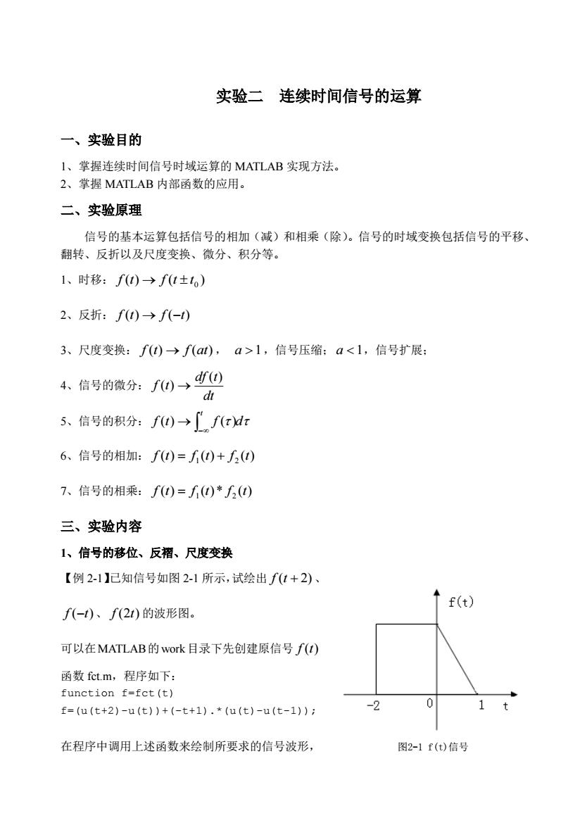
信号与系统实验指导书 f1+2) 1.5 5 时间 时间 05 时间: 时间: 图2-2信号的移位、反折、尺度变换 2、信号的微分、积分 【例2-2】用MATLAB命令绘制信号∫()=sin(wI))的一阶微分信号及一阶积分信号. 程序如下: syms y yl y2t v=sin(w*t): subplot(311) ezplot(y) yl=diff(y.'t): %信号微分 subplot(312) ezplot(y1) y2=imty1,t),%信号积分 subplot(313) ezplot(y2) 程序运行后,波形如图2-3所示
信号与系统实验指导书 -2- 2、信号的微分、积分 【例 2-2】用 MATLAB 命令绘制信号 f (t) sin(wt) 的一阶微分信号及一阶积分信号。 程序如下: syms y y1 y2 t y=sin(w*t); subplot(311) ezplot(y) y1=diff(y,'t'); %信号微分 subplot(312) ezplot(y1) y2=int(y1,'t'); %信号积分 subplot(313) ezplot(y2) 程序运行后,波形如图 2-3 所示。 图 2-2 信号的移位、反折、尺度变换
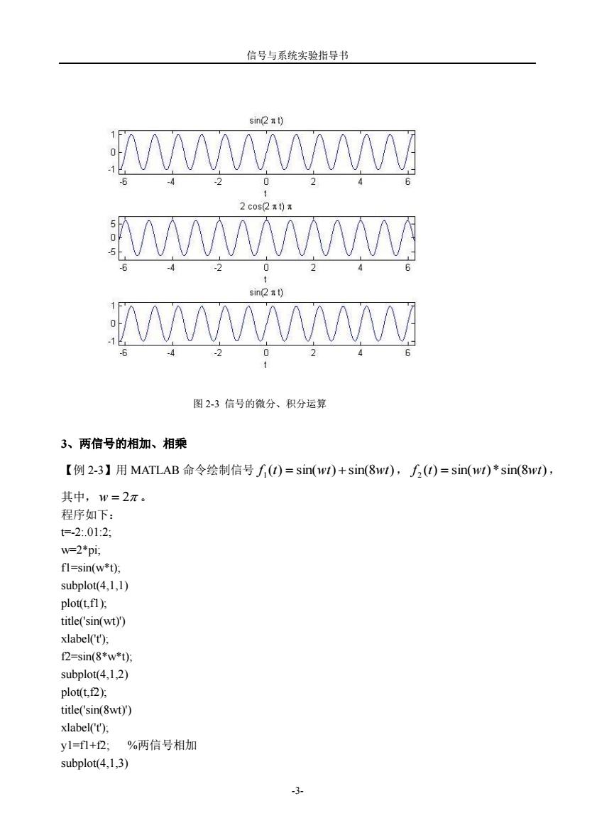
信号与系统实验指导书 N 2 WMWW☑ sin2 t) MW 0 图2-3信号的微分、积分运算 3、两信号的相加、相乘 【例2-3】用MATLAB命令绘制信号f)=sin(wI)+sin(8w),5()=sin(w)*sim(8wI), 其中,w=2π。 程序如下: te-2:.012: w=2*pi; fl=sin(w*t); subplot(4.1.1) plot(t.fl)方 title('sin(wt)) xlabel(t). f2=sin(8*w*t); subplot(4.1.2) plot(t,2); title(sin(8wt)) xlabel('t); y1=f1+2 %两信号相加 subplot(4,1,3)
信号与系统实验指导书 -3- 3、两信号的相加、相乘 【例 2-3】用 MATLAB 命令绘制信号 ( ) sin( ) sin(8 ) f 1 t wt wt , ( ) sin( )*sin(8 ) f 2 t wt wt , 其中, w 2 。 程序如下: t=-2:.01:2; w=2*pi; f1=sin(w*t); subplot(4,1,1) plot(t,f1); title('sin(wt)') xlabel('t'); f2=sin(8*w*t); subplot(4,1,2) plot(t,f2); title('sin(8wt)') xlabel('t'); y1=f1+f2; %两信号相加 subplot(4,1,3) 图 2-3 信号的微分、积分运算

信号与系统实验指导书 plot(ty)方 title('sin(wt)+sin(8wt)) xlabel(t). y1=f1.*2; 两信号相乘 subplot(4.1.4) plot(tyl). title('sin(wt)*sin(8wt)) xlabel('t); 程序运行后,波形如图2-4所示。 sin(wt) .15 105 0 0.5 15 sin(8wt) .1.5 0.5 0.5 sin(wt)+sin(Bwt) wwwwwwwwwww 2-1.5 105 00.5 11.5 sin(wt)"sin(8wt) WNwwWwW .15 .1 -0.5 0 0.5 1 15 t 图2-4两信号的相加、相乘 4、信号的奇偶分解 【例2-1】已知信号f0)=sn号u(0-1-2训,试绘出信号f0的偶分量和奇分量. 程序如下: =2:.012 f=sin(pi*t/2).*(u(t)-u(t-2)). subplot(31l); plot(t,f); grid on title('f(t)); xlabel('时间t)
信号与系统实验指导书 -4- plot(t,y1); title('sin(wt)+sin(8wt)') xlabel('t'); y1=f1.*f2; %两信号相乘 subplot(4,1,4) plot(t,y1); title('sin(wt)*sin(8wt)') xlabel('t'); 程序运行后,波形如图 2-4 所示。 4、信号的奇偶分解 【例 2-1】已知信号 [ ( ) ( 2)] 2 f (t) sin t u t u t ,试绘出信号 f (t) 的偶分量和奇分量。 程序如下: t=-2:.01:2; f=sin(pi*t/2).*(u(t)-u(t-2)); subplot(311); plot(t,f); grid on title('f(t)'); xlabel('时间 t'); 图 2-4 两信号的相加、相乘