
1.3 Some Useful Signal Operations b4 1 Introduction to Signals and Systems -2 f(2) 3 2 Plg-1.12 Time inversion (refection)of a signal 2e-4 2 -1.5s<0ow-3st<0 =1(偵={2e- 0≤<3or0≤t<6 (1186) 10 6 Observe that the instantst-1.5 and 3nf()correspond to the instantst=-3and 6 in the expanded aignal(》.■ Fig.1.11 (s)signal f(t)(b)signal (3)(c)signal() △Exercis0E1.& ■Example1.4 Show that the() Figure 1.11a hows a sigal/(t).Sketch and describe me amplitude and phase,but with the frequenry and phase but with time-compresed by factor 3.Repent the problem for gnal time-expanded by b a faetor n(n>1)of a sinusaid ree In a sinu ctdpded tuctoe 2 2 -15≤t<0 f)={2e- 0st<3 (117 1.3-3 Time Inversion (Time Reversal) Comsider the)in We()re at the ertical axis.To time-invert f(t),we rotate this frame 18 oout the right-hand side of Eo.1.7.Thus somo instant tal happens in Fig.1.12b at the instant us the signal)(Fig.1.12b).Observe that whate ver 2 -1.5≤3<0ar-0.5≤t<0 (-)=fe) f()=f3) 了2e-3n 0≤3t<3or0≤【<1 (1.18a) and 40 otherwise )=f-) (1.19) -1.5 and 3 in f(correspond to the instantst=05,and 1 in the compressed Terfore,to time-invertgThhoo ror image of f(t)about the vertical dercrbedmtbe5yaoa.hootaned/为ih。 Figure 1. which is f(t)time-expanded by factor 2:cons off(t)about the horizontal axis is m -je)
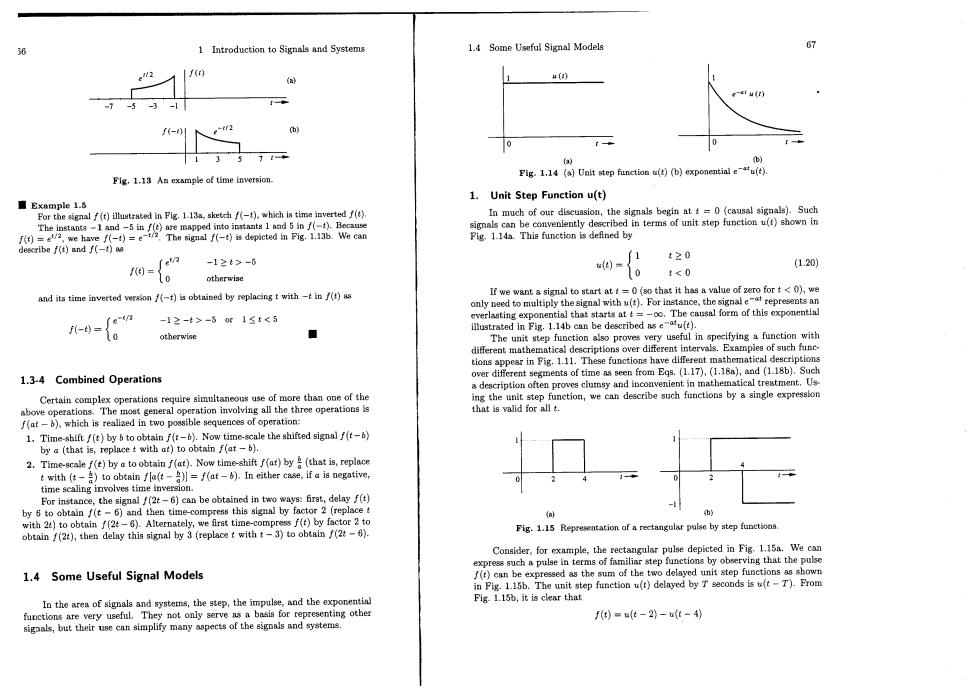
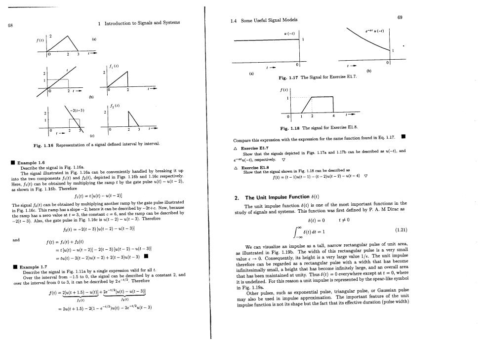
1 Introduction to Signals and Systems 1.4 Some Useful Signal Models f er u(r) -3-1 137 (a) Flg.1.13 An example of time inversion. sgi4周Ve h的间expoial-e 1.Unit Step Function u(t) ■Example 1.5 For the sgalf(t)illustrated in Fig.1.13m,sketch f),which is time inverted f() h of the n att=0 (causal signals).Such 1t20 0=0 -12t3-6 (1.20) otherwise <0 and its time inverted veraonf()is obtained by replacingt with-tin()as rwewantaignltotartatt=0(eethatthsaaeoft fort<0以,we only need to multiply the aignal with (t).For in nce,th of this no-fon -12->-515t<5 50 otherwise ■ The unit step also proves riptions over different mathematical descriptions 1.3-4 Combined Operations Eos ()(1.18s),and(118b).Such on often prow d ip Certain complex operations require simultaneous use of more than one of the above operations.The most general operation involving all the three operations is f(at-),which is reallized in two possible sequences of operation: 1.Time-shift f()by b toobtainf().Now time-scale the shifted signal f( by a(that is,)to obtain f(b). 2.Time-abytobtain f(at).Now tim-hift (a)by( twith (t)to obtain fla(t)]=f(at-).In either case,if a is negative, time scaling involves time inversion. For instace the signal6)be obtained inwaysfirst,delay( 如oeRe8gAa b) f(t)by la obtain f(2e),then delay this signal by 3 (replace t with t-3)to obtain f(2t- Pig.1.15 Representation of rectangular pulse by step function Consider,for example,the rectangular pulse depicted in Fig-1.15a.We can lse in terms of familiar step functions by observing that the pulse 1.4 Some Useful Signal Models f(t)can be expressed as the sum of the two delayed unit step functions as shown in Pig.1.15b.The unit step function u(t)delayed by T seconds is u(t-T).From Pig-1.15b,it is clear that e other are very useful.They not only serve as a basis for representing other f)=wt-2)-4)
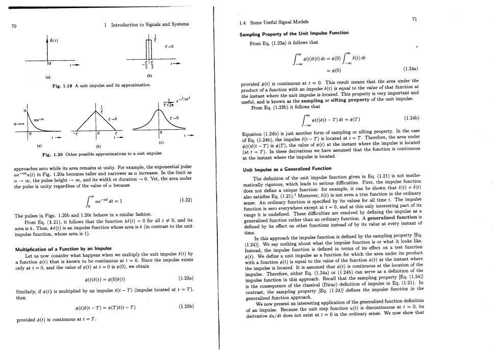
1 Introduction to Signals and Systems 1.4 Some Useful Signal Models Fig.1.17 The Signal for Exercise E1.7. Flg.1.18 The signal for Exercise E1.8. Fig.1.16 Representatlon of a signal defined interval by interval. Compare this expreasion with the expression for the same function found in E1.17. △Ex relso E1,T Show that the sigals deplcted in Pigs.1.17a and 1.1Tb ckn be deacribeds)and ee Example1.6 e-afu(-),reapectively. The signal illustrate eniently handled by breaking it up ghoin be dbed cted in Figs.1.16b and 1.16c respectively f=t-10ut-)-t-2u(t-2-ut-497 h(=tu()-t-2明 2.The Unit Impulse Function 6(t) ortant functions in the inrap haa lope hect can be descib 6)■0 *0 f0=-2t-3)ut-2)-ut-3别 (1.21) and f(0=)+因 tall.n row rectangular pulse of unit area =t(0-u(t-2)-2t-3)u(t-2)-u(t-3别 th of this rectangular pulse is a very smal =0-3e-2)4t-2)+2t-3ju(t-3)■ value0.Consequently,its hei large value 1/e.The unit impulse therefore can be regard signal in Fig.1.11a by a single expression valid for allt. e my that has beer d at V.Thus 6(t)0everywhere except att=0,whe it is unden ed.For s represented by the spear-like symbo e=2t+15)-0+22=0-t-3到 in Fig.1.19a. Other puls such as ponential pulse,triangular pulse,or Gaussiar n pulse roximation.The important feature of h =2ut+1.5-21-en)u0-2e-nut-3)
1 Introduction to Signals and Systems 1.4 Some Useful Signal Models Sampling Property of the Unit Impulse Function From Eq.(1.23a)it follows that 严ses日=4o广s0a =(0) (1.24a) (b) Fig.1.10 A unit impulse and its approximation. whe and 2 e-le From Eq.(1.23b)it follows that 广ee-a=sm 1.24bj Equation (1.24b)is just another form operty.In the case e T)ocateTherefore,the rea under fe) tant where the impulse is located Fig.1.20 Other poseible approximation tounit impulse (at t=T).In these derivati approcero while tsareanityFor theexponu t or ratio Yathe Unit Impulse as a Generalized Function ac does not de 1.22) also satisfies Bg、1.21jMo er.6(t)is not even a true function in the ordinary sense.An ordinary fun is specified by its values for all time t.The impul pt at t0,and at this only intere ting part of it The pulses in Figs.1.20b and 1.20c behave in asmla fashion range1t ather than an ordinary function.A generali byitoher functodof byitvaueeve time In this app onch the impuise function is defined by the sa (1.24月 othing about what the impulse function Multiplication of a Function by an Impulse )Weleme mpunctin for on a test function h a function (is equal to the value of the function only at t=0.and the value of (t)at t=0 is(0),we obtain located.It is assumed that the ocation of the Therefore,either Eq.(1.24a)or adefinition of the 24b)can serv (d)6fe)=(0)6(t) (1.23a oulse function in this approach.Recall tyE.(1.24 is the copsequence of the classical(Dirac (121.n Smilarly,if)is multiplied by an impulse(t-T)(impulse located att=T). contrast,the sampling property Eq.(124)defines the impulse function in the then generalized function appronch. ralized function definition )6t-T)=(T)t-T) (1.23b) We now present an interesting appli cation of the ( at t=0 its provided is continuous at=T
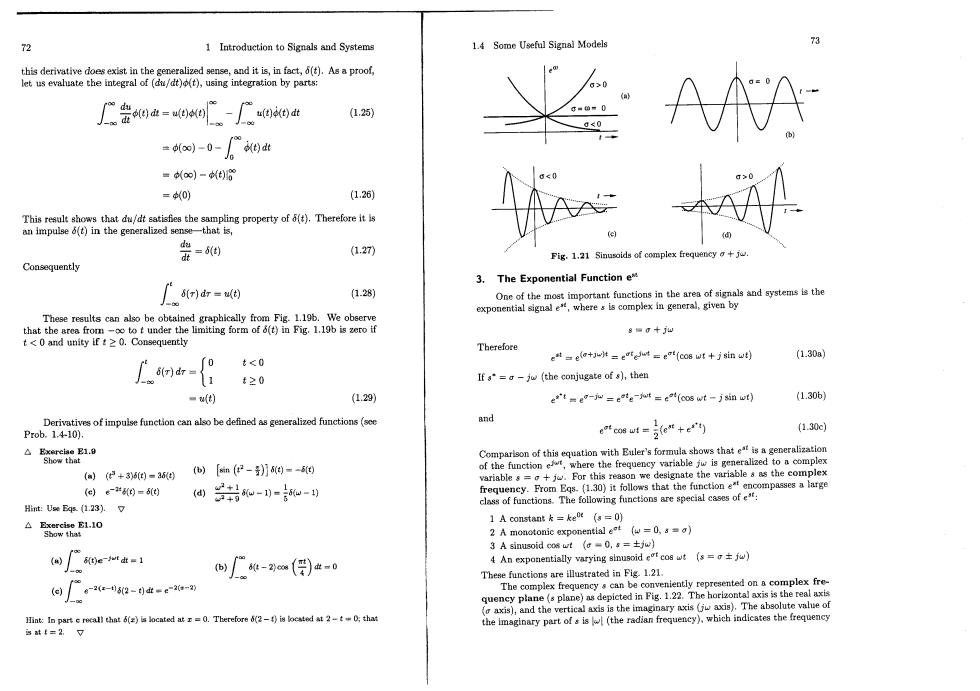
1 Introduction to Signals and Systems 1.4 Some Useful Signal Models this derivative does exist in the generalized sens,and it is,in fact,(t).Asa proof, let us evalate the integral of (du/dt)(t),using integration by parts: (1.25) 0<0 A的 -0-的 =∞)-t)8 =0) (1.26) This reault shows ling property of().Thereforet =sid (1.27) Fig.1.1 Sinusoids of complex frequenc Consequently 3.The Exponential Function e 「r)dr=4) (1.28) ne of the complex in general,given by Thesee be obtained graphically from Fig1.19b.Webeerve that the otot under the limiting form of (t)in Fig.1.19b is zero if 8eg十jw Therefore et=e(a+=et=et (co8 wt+jsin wt) (1.30a) ft-日 t<0 If s"=a-jw (the conjugate of s),then ■( (1.29) e'te-jw =eate-jwit e (cos wt -jsin wt) (1.306) Derivatives of impulse function can so be defined as generalized functions (se and Prob.1.410). oco wt(e (1.30e △c1-0 o)(2+38g-a6g【m(2-月g-阳 variable s =+j.For this reason we d (e)6-#60= 间w-和- Hint:Use Egs.(1.23). △BeeE1-1o 1 A constant k =ke0t (s=0) 2 A monotonic exponential et (w=0.s=) 3 A sinusoid t(-0,s=±ow) o广s0e-wtk- -(月) 4 An exponentially varying sinusoid et coswt (s=) These functions are illustrated in Fig 1.21. 。u-80-0a-e20- The lex fr be conveniently represented ona complex fre lane (s plane)ns depicted in Fig.1.22.The horizontal axi s).and the vertical axis is the imaginary axis (w axis ute vale Hint:In part ercall that (is located at=0.Therefore(2-f)is located at t:tha the ofis(the radian frequency)which indicates the is at I=2.V