
then will give a feel for the properties of the scalar function.We show such a contour map in the xy-plane atz=0 for Eq.(1.2.2),namely, 1 1/3 (x,y,0)= (1.2.3) Vx2+y+d2Vx2+y-d0月 Various contour levels are shown in Figure 1.2.4,for d=1,labeled by the value of the function at that level. -2 0 Figure 1.2.4 A contour map in the xy-plane of the scalar field given by Eq.(1.2.3). 2.Color-Coding Another way we can represent the values of the scalar field is by color-coding in two dimensions for a fixed value of the third.This was the scheme used for illustrating the temperature fields in Figures 1.2.1 and 1.2.2.In Figure 1.2.5 a similar map is shown for the scalar field (x,y,0).Different values of (x,y,0)are characterized by different colors in the map. 0 2 0 21 Figure 1.2.5 A color-coded map in the xy-plane of the scalar field given by Eq.(1.2.3). 1-6
1-6 then will give a feel for the properties of the scalar function. We show such a contour map in the xy-plane at z = 0 for Eq. (1.2.2), namely, ( ) ( ) 2 2 2 2 1 1/3 ( , ,0) x y x yd x yd φ = − ++ +− (1.2.3) Various contour levels are shown in Figure 1.2.4, for d =1, labeled by the value of the function at that level. Figure 1.2.4 A contour map in the xy-plane of the scalar field given by Eq. (1.2.3). 2. Color-Coding Another way we can represent the values of the scalar field is by color-coding in two dimensions for a fixed value of the third. This was the scheme used for illustrating the temperature fields in Figures 1.2.1 and 1.2.2. In Figure 1.2.5 a similar map is shown for the scalar field ( , ,0) φ x y . Different values of ( , ,0) φ x y are characterized by different colors in the map. Figure 1.2.5 A color-coded map in the xy-plane of the scalar field given by Eq. (1.2.3)
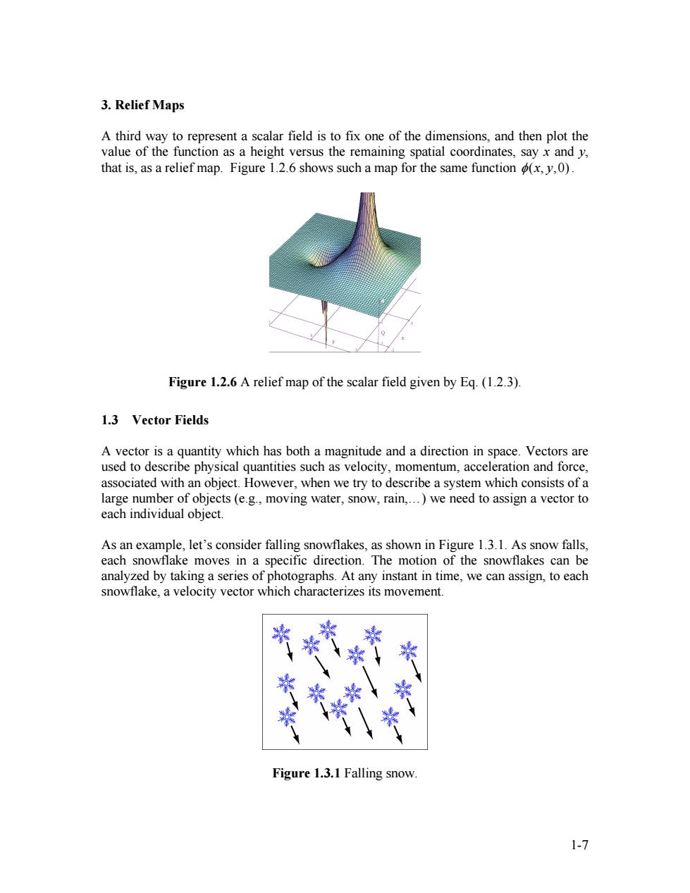
3.Relief Maps A third way to represent a scalar field is to fix one of the dimensions,and then plot the value of the function as a height versus the remaining spatial coordinates,say x and y, that is,as a relief map.Figure 1.2.6 shows such a map for the same function (x,y,0). Figure 1.2.6 A relief map of the scalar field given by Eq.(1.2.3). 1.3 Vector Fields A vector is a quantity which has both a magnitude and a direction in space.Vectors are used to describe physical quantities such as velocity,momentum,acceleration and force, associated with an object.However,when we try to describe a system which consists of a large number of objects (e.g.,moving water,snow,rain,...)we need to assign a vector to each individual object. As an example,let's consider falling snowflakes,as shown in Figure 1.3.1.As snow falls, each snowflake moves in a specific direction.The motion of the snowflakes can be analyzed by taking a series of photographs.At any instant in time,we can assign,to each snowflake,a velocity vector which characterizes its movement. Figure 1.3.1 Falling snow. 1-7
1-7 3. Relief Maps A third way to represent a scalar field is to fix one of the dimensions, and then plot the value of the function as a height versus the remaining spatial coordinates, say x and y, that is, as a relief map. Figure 1.2.6 shows such a map for the same function ( , ,0) φ x y . Figure 1.2.6 A relief map of the scalar field given by Eq. (1.2.3). 1.3 Vector Fields A vector is a quantity which has both a magnitude and a direction in space. Vectors are used to describe physical quantities such as velocity, momentum, acceleration and force, associated with an object. However, when we try to describe a system which consists of a large number of objects (e.g., moving water, snow, rain,…) we need to assign a vector to each individual object. As an example, let’s consider falling snowflakes, as shown in Figure 1.3.1. As snow falls, each snowflake moves in a specific direction. The motion of the snowflakes can be analyzed by taking a series of photographs. At any instant in time, we can assign, to each snowflake, a velocity vector which characterizes its movement. Figure 1.3.1 Falling snow
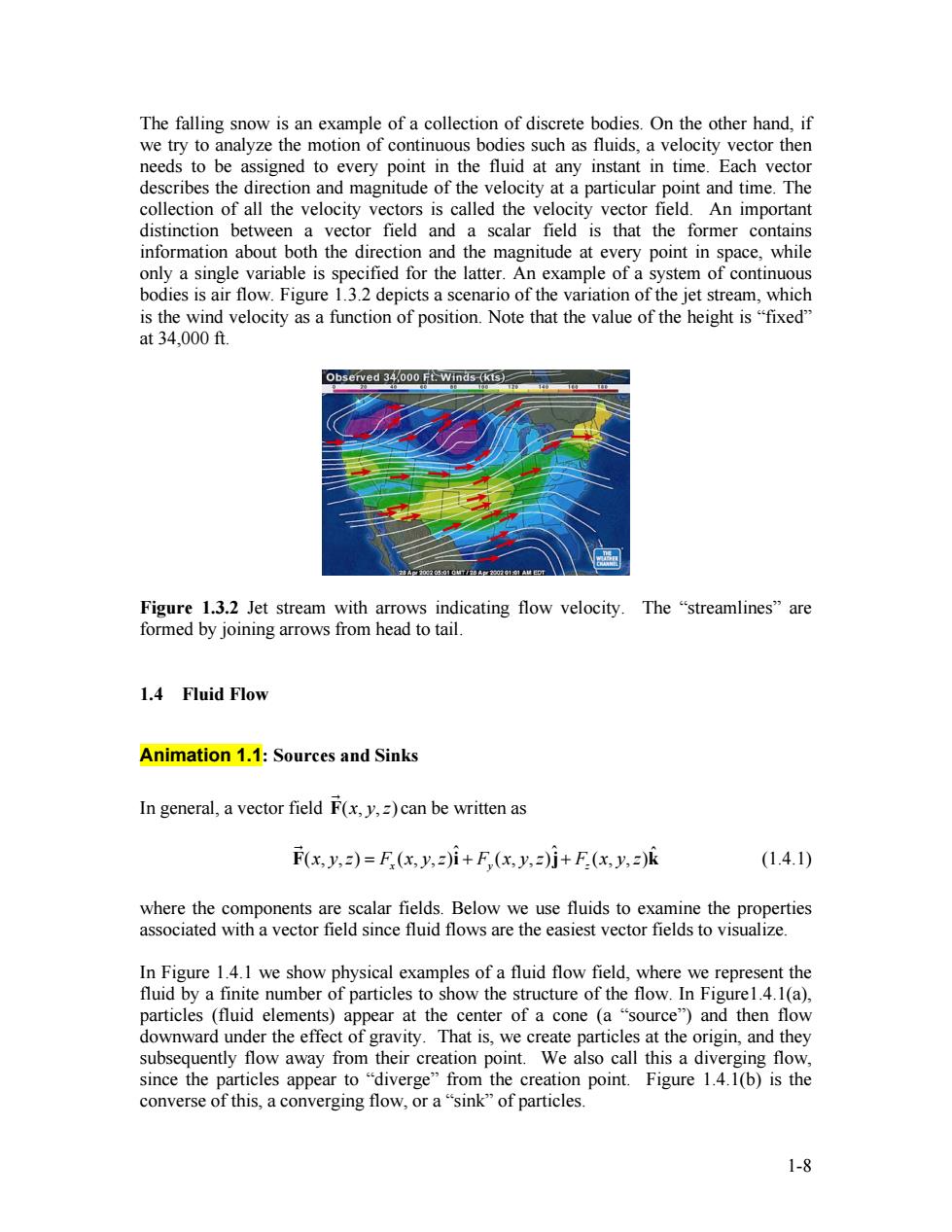
The falling snow is an example of a collection of discrete bodies.On the other hand,if we try to analyze the motion of continuous bodies such as fluids,a velocity vector then needs to be assigned to every point in the fluid at any instant in time.Each vector describes the direction and magnitude of the velocity at a particular point and time.The collection of all the velocity vectors is called the velocity vector field.An important distinction between a vector field and a scalar field is that the former contains information about both the direction and the magnitude at every point in space,while only a single variable is specified for the latter.An example of a system of continuous bodies is air flow.Figure 1.3.2 depicts a scenario of the variation of the jet stream,which is the wind velocity as a function of position.Note that the value of the height is "fixed" at34,000ft. Observed 34,000 Ft.Winds (kts) Figure 1.3.2 Jet stream with arrows indicating flow velocity.The "streamlines"are formed by joining arrows from head to tail. 1.4 Fluid Flow Animation 1.1:Sources and Sinks In general,a vector field F(x,y,)can be written as F(x.y,=)=F(x.y,=)i+F(x.y,=)j+F(x.y,2)k (1.4.1) where the components are scalar fields.Below we use fluids to examine the properties associated with a vector field since fluid flows are the easiest vector fields to visualize In Figure 1.4.1 we show physical examples of a fluid flow field,where we represent the fluid by a finite number of particles to show the structure of the flow.In Figure1.4.1(a), particles (fluid elements)appear at the center of a cone (a "source")and then flow downward under the effect of gravity.That is,we create particles at the origin,and they subsequently flow away from their creation point.We also call this a diverging flow, since the particles appear to "diverge"from the creation point.Figure 1.4.1(b)is the converse of this,a converging flow,or a "sink"of particles. 1-8
1-8 The falling snow is an example of a collection of discrete bodies. On the other hand, if we try to analyze the motion of continuous bodies such as fluids, a velocity vector then needs to be assigned to every point in the fluid at any instant in time. Each vector describes the direction and magnitude of the velocity at a particular point and time. The collection of all the velocity vectors is called the velocity vector field. An important distinction between a vector field and a scalar field is that the former contains information about both the direction and the magnitude at every point in space, while only a single variable is specified for the latter. An example of a system of continuous bodies is air flow. Figure 1.3.2 depicts a scenario of the variation of the jet stream, which is the wind velocity as a function of position. Note that the value of the height is “fixed” at 34,000 ft. Figure 1.3.2 Jet stream with arrows indicating flow velocity. The “streamlines” are formed by joining arrows from head to tail. 1.4 Fluid Flow Animation 1.1: Sources and Sinks In general, a vector field F(, ,) x y z G can be written as ˆ ˆ ˆ (, ,) (, ,) (, ,) (, ,) xyz F i x yz F xyz F xyz F xyz =++j k G (1.4.1) where the components are scalar fields. Below we use fluids to examine the properties associated with a vector field since fluid flows are the easiest vector fields to visualize. In Figure 1.4.1 we show physical examples of a fluid flow field, where we represent the fluid by a finite number of particles to show the structure of the flow. In Figure1.4.1(a), particles (fluid elements) appear at the center of a cone (a “source”) and then flow downward under the effect of gravity. That is, we create particles at the origin, and they subsequently flow away from their creation point. We also call this a diverging flow, since the particles appear to “diverge” from the creation point. Figure 1.4.1(b) is the converse of this, a converging flow, or a “sink” of particles
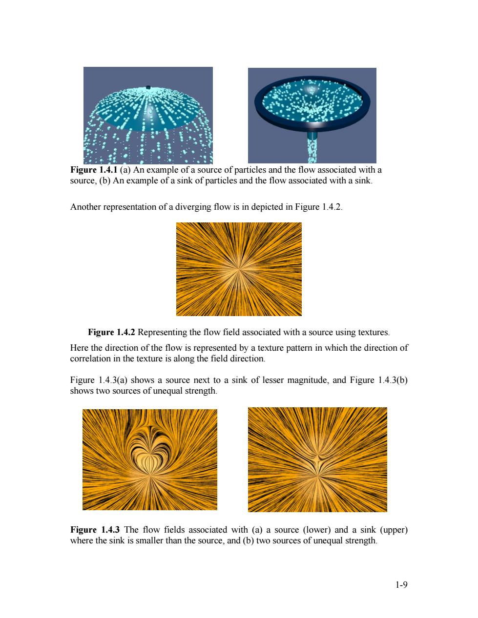
Figure 1.4.1 (a)An example of a source of particles and the flow associated with a source,(b)An example of a sink of particles and the flow associated with a sink. Another representation of a diverging flow is in depicted in Figure 1.4.2. Figure 1.4.2 Representing the flow field associated with a source using textures. Here the direction of the flow is represented by a texture pattern in which the direction of correlation in the texture is along the field direction. Figure 1.4.3(a)shows a source next to a sink of lesser magnitude,and Figure 1.4.3(b) shows two sources of unequal strength. Figure 1.4.3 The flow fields associated with (a)a source (lower)and a sink (upper) where the sink is smaller than the source,and (b)two sources of unequal strength. 1-9
Figure 1.4.1 (a) An example of a source of particles and the flow associated with a source, (b) An example of a sink of particles and the flow associated with a sink. Another representation of a diverging flow is in depicted in Figure 1.4.2. Figure 1.4.2 Representing the flow field associated with a source using textures. Here the direction of the flow is represented by a texture pattern in which the direction of correlation in the texture is along the field direction. Figure 1.4.3(a) shows a source next to a sink of lesser magnitude, and Figure 1.4.3(b) shows two sources of unequal strength. Figure 1.4.3 The flow fields associated with (a) a source (lower) and a sink (upper) where the sink is smaller than the source, and (b) two sources of unequal strength. 1-9