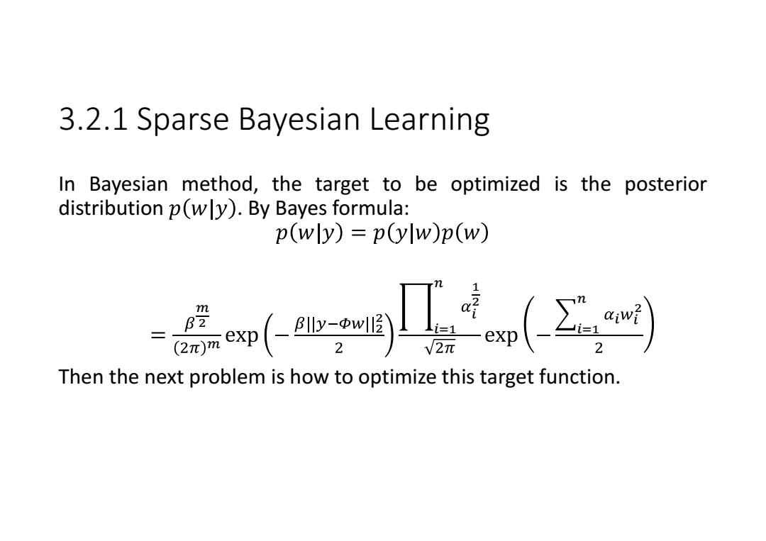
3.2.1 Sparse Bayesian Learning In Bayesian method,the target to be optimized is the posterior distribution p(wly).By Bayes formula: p(wly)=p(ylw)p(w) wnf m = Then the next problem is how to optimize this target function
3.2.1 Sparse Bayesian Learning In Bayesian method, the target to be optimized is the posterior distribution . By Bayes formula: మ మ మ భ మ సభ మ సభ Then the next problem is how to optimize this target function
3.3.1 EM algorithm To find a convergent algorithm to optimize the target function,we first introduce the expectation maximization algorithm. The expectation maximization algorithm,or EM algorithm,is a general technique for finding maximum likelihood solutions for probabilistic models having latent variables It is formal introduced in 1977 by Dempster et al.,"Maximum likelihood from imcomplete data via the EM algorithm". The first publications in IEEE journals making reference to the EM algorithm appeared in 1988 and dealt with the problem of tomographic reconstruction of photon limited images. Since then,the EM algorithm has become a popular tool for statistical signal processing used in a wide range of applications
3.3.1 EM algorithm To find a convergent algorithm to optimize the target function, we first introduce the expectation maximization algorithm. • The expectation maximization algorithm, or EM algorithm, is a general technique for finding maximum likelihood solutions for probabilistic models having latent variables • It is formal introduced in 1977 by Dempster et al., "Maximum likelihood from imcomplete data via the EM algorithm". • The first publications in IEEE journals making reference to the EM algorithm appeared in 1988 and dealt with the problem of tomographic reconstruction of photon limited images. • Since then, the EM algorithm has become a popular tool for statistical signal processing used in a wide range of applications
3.3.1 EM algorithm We first introduce two concepts. 1.Observed variables:the variables that are observed:like y in y w +e,we know the values of the variables. 2.Hidden/latent variables:the values are unobserved but their values affects the observed variables.Like w in y =w +e. EM algorithm:to find the optimal parameters in a system with hidden variables
3.3.1 EM algorithm We first introduce two concepts. 1. Observed variables: the variables that are observed: like , we know the values of the variables. 2. Hidden/latent variables: the values are unobserved but their values affects the observed variables. Like in . EM algorithm: to find the optimal parameters in a system with hidden variables
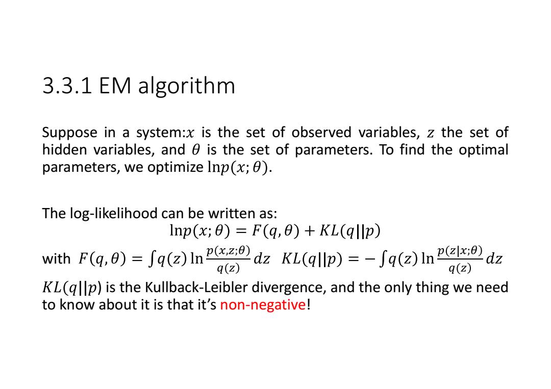
3.3.1 EM algorithm Suppose in a system:x is the set of observed variables,z the set of hidden variables,and 0 is the set of parameters.To find the optimal parameters,we optimize Inp(x;) The log-likelihood can be written as: Inp(x;0)=F(q,0)+KL(qllp) with F(q,0)=Sq(z)Indz KL(qllp)=-Sq(z)In dz q(z) q(z) KL(gp)is the Kullback-Leibler divergence,and the only thing we need to know about it is that it's non-negative!
3.3.1 EM algorithm Suppose in a system: is the set of observed variables, the set of hidden variables, and is the set of parameters. To find the optimal parameters, we optimize . The log-likelihood can be written as: with ) is the Kullback-Leibler divergence, and the only thing we need to know about it is that it’s non-negative!
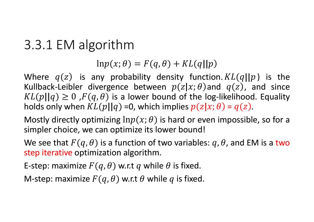
3.3.1 EM algorithm Inp(x;0)=F(q,0)+KL(qllp) Where q(z)is any probability density function.KL(qp)is the Kullback-Leibler divergence between p(zx;)and q(z),and since KL(pllq)≥0,F(q,θ)is a lower bound of the log--likelihood.Equality holds only when KL(pq)=0,which implies p(zx;0)=q(z). Mostly directly optimizing Inp(x;0)is hard or even impossible,so for a simpler choice,we can optimize its lower bound! We see that F(g,0)is a function of two variables:g,0,and EM is a two step iterative optimization algorithm. E-step:maximize F(q,)w.r.t q while 0 is fixed. M-step:maximize F(q,0)w.r.t 0 while g is fixed
3.3.1 EM algorithm Where is any probability density function. ) is the Kullback-Leibler divergence between and , and since , is a lower bound of the log-likelihood. Equality holds only when =0, which implies = . Mostly directly optimizing is hard or even impossible, so for a simpler choice, we can optimize its lower bound! We see that is a function of two variables: , and EM is a two step iterative optimization algorithm. E-step: maximize w.r.t while is fixed. M-step: maximize w.r.t while is fixed