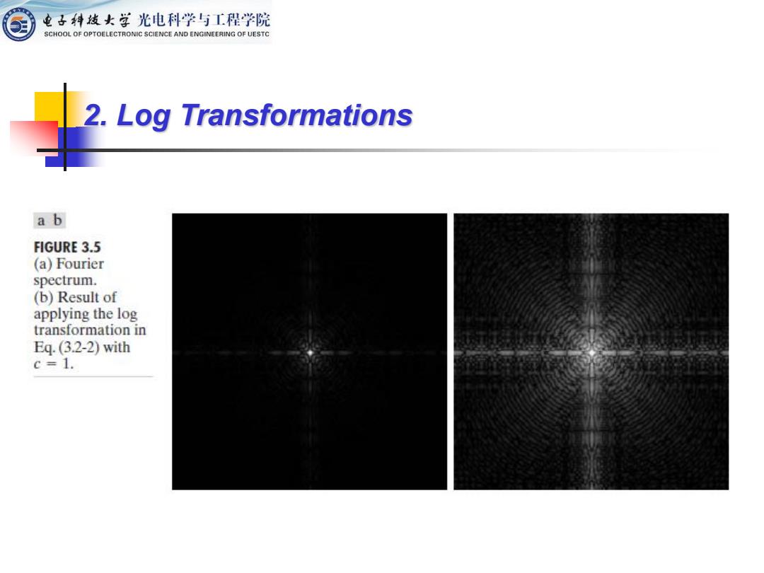
电子科线女学光电科学与工程学院 SCHOOL OF OPTOELECTRONIC SCIENCE AND ENGINEERING OF UESTC 2.Log Transformations ab FIGURE 3.5 (a)Fourier spectrum. (b)Result of applying the log transformation in Eq.(3.2-2)with c=1
2. Log Transformations

电子科发女学光电科学与工程学院 SCHOOL OF OPTOELECTRONIC SCIENCE AND ENGINEERING OF UESTC 3.Power-Law Transformations L-1 y=0.04 y=0.10 3L/4 y=020 ■where c and r are y=0.40 positive constant. y=0.67 Sometimes it is written L/2 y=1 as s=c(r+). indino y=1.5 FIGURE 3.6 Plots y=2.5 of the equation L/4 y=5.0 s =crY for various values of y=10.0 y (c 1 in all y=25.0 cases).All curves were scaled to fit 0 L/4 L/2 3L/4 L-1 in the range Input intensity level,r shown
3. Power-Law Transformations s cr = ◼ where c and r are positive constant. Sometimes it is written as . s c r( ) = +
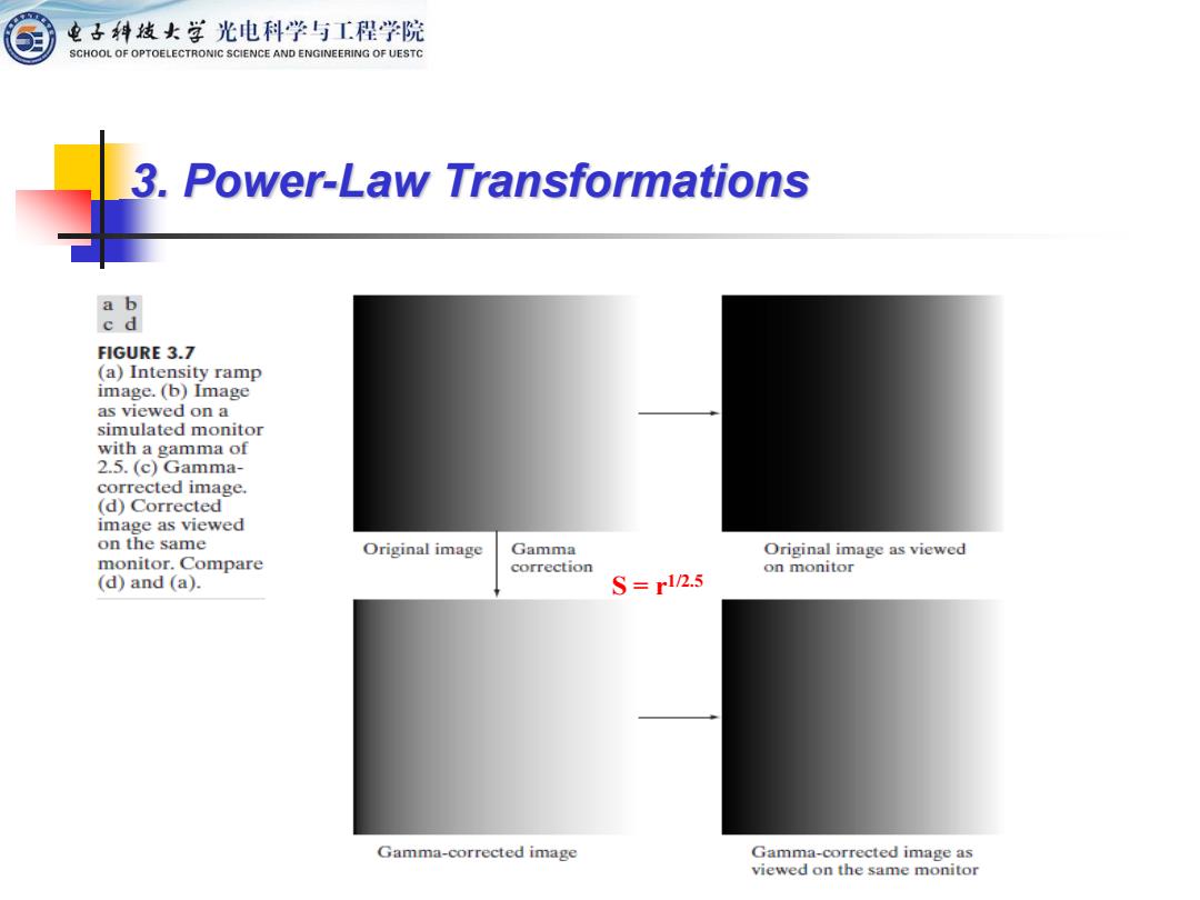
电子科发女学光电科学与工程学院 SCHOOL OF OPTOELECTRONIC SCIENCE AND ENGINEERING OF UESTC 3.Power-Law Transformations a b cd FIGURE 3.7 (a)Intensity ramp image.(b)Image as viewed on a simulated monitor with a gamma of 2.5.(c)Gamma- corrected image. (d)Corrected image as viewed on the same Original image Gamma Original image as viewed monitor.Compare correction on monitor (d)and (a). S=r12.5 Gamma-corrected image Gamma-corrected image as viewed on the same monitor
3. Power-Law Transformations S = r1/2.5

电子科线女学光电科学与工程学院 SCHOOL OF OPTOELECTRONIC SCIENCE AND ENGINEERING OF UESTC 3.Power-Law Transformations a b cd FIGURE 3.8 (a)Magnetic resonance image (MRI of a fractured human spine. (b)-(d)Results of applying the transformation in Eq.(3.2-3)with c I and y=0.6.04and 0.3,respectively. (Original image courtesy of Dr. David R.Pickens. Department of Radiology and Radiological Sciences. Vanderbilt University Medical Center.)
3. Power-Law Transformations

电子科发女学光电科学与工程学院 SCHOOL OF OPTOELECTRONIC SCIENCE AND ENGINEERING OF UESTC 3.Power-Law Transformations cd FIGURE 3.9 (a)Acrial image. (b)-(d)Results of applying the transformation in Eq.(3.2-3)wih c=1and y=3.0.4.0.and 5.0.respectively. (Original image for this example courtesy of NASA.)
3. Power-Law Transformations