0122229现代数字通信与编码理论 September 1,2022 XDU,Fall 2022 Lecture Notes Chapter 2 Modulation and Coding for Ideal Gaussian channels This chapter is devoted to the discussion on orthonormal PAM/QAM systems,capacity calculations for ideal AWGN channels,and the performance evaluation of small signa constellations Note:Some of material presented in this chapter is based on Forney's lecture notes. 2.1 Data modulation and Demodulation In data modulation we c onvert information bits into waveforms that are suitable for transmission over a communication channel. This is done,in general,by splitting data modulation(or channel encoding)into separate layers:mapping from a sequence of binary digits into a sequence of real or complex numbers (numerical signals),followed by the conversion of signals to a waveform.Demodulation is the corresponding process at the ece maps the received waveform to a sequence of received signals In a passband system,modulators usually include a third layer,which maps a baseband-encoded waveform()into a passband wavefor(( with carrier frequencyf.At the receiver this passband waveform is mapped back to aseband ning the other components of decoding.This frequency conversion operation at encoder and decoder is often referred to as modulation and demodulation,but it is more common today to use the word modulation for the entire process of mapping bits to waveforms.Figure 2.0 illustrates these three layers. Binary Bits to Signals to Baseband to Input signals waveform passband of baseband pas an Channel waveform Binary Signal Waveform Passband to Output decoder to signals baseband Figure 2.0 The layers of a modulator (channel encoder)and demodulator (channel decoder) 2.1.1 Mapping of vectors to waveform It is well-known that any continuous-time function x()C defined on the interval [0. T]can be decomposed according to some set of N orthonormal basis function (t),Isks 2-1
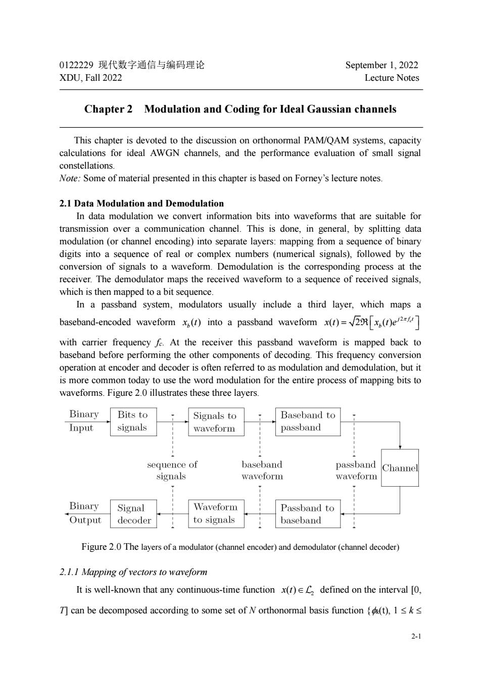
2-1 0122229 现代数字通信与编码理论 September 1, 2022 XDU, Fall 2022 Lecture Notes Chapter 2 Modulation and Coding for Ideal Gaussian channels This chapter is devoted to the discussion on orthonormal PAM/QAM systems, capacity calculations for ideal AWGN channels, and the performance evaluation of small signal constellations. Note: Some of material presented in this chapter is based on Forney’s lecture notes. 2.1 Data Modulation and Demodulation In data modulation we convert information bits into waveforms that are suitable for transmission over a communication channel. This is done, in general, by splitting data modulation (or channel encoding) into separate layers: mapping from a sequence of binary digits into a sequence of real or complex numbers (numerical signals), followed by the conversion of signals to a waveform. Demodulation is the corresponding process at the receiver. The demodulator maps the received waveform to a sequence of received signals, which is then mapped to a bit sequence. In a passband system, modulators usually include a third layer, which maps a baseband-encoded waveform () b x t into a passband waveform 2 ( ) 2 ( ) c j f t b x t x t e = R with carrier frequency fc. At the receiver this passband waveform is mapped back to baseband before performing the other components of decoding. This frequency conversion operation at encoder and decoder is often referred to as modulation and demodulation, but it is more common today to use the word modulation for the entire process of mapping bits to waveforms. Figure 2.0 illustrates these three layers. Figure 2.0 The layers of a modulator (channel encoder) and demodulator (channel decoder) 2.1.1 Mapping of vectors to waveform It is well-known that any continuous-time function 2 x t( ) defined on the interval [0, T] can be decomposed according to some set of N orthonormal basis function {k(t), 1 k
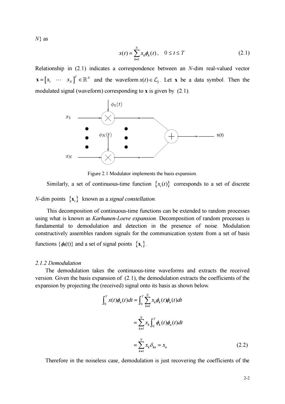
N)as 0-2400s1s7 2.10 Relationship in (2.1)indicates a correspondence between an N-dim real-valued vector x=[x.xxER and the waveformx(r)eC.Let x be a data symbol.Then the modulated signal(waveform)corresponding tox is given by (2.1). (t) ● ON() ● N Figure Modulator the basis expansion. Similarly,a set of continuous-time function()corresponds to a set of discrete N-dim pointsx known as a signal constellation. ous-time functions can be extended to random processes using what is known as Karhunen-Loeve expansion.Decomposition of random processes is fundamental to demodulation and detection in the presence of noise.Modulation constructively assembles random signals for the communication system from a set of basis functions())and a set of signal pointsx 2.1.2 Demodulation The demodulation takes the continuous-time waveforms and extracts the received version.Given the basis expansion of(2.1),the demodulation extracts the coefficients of the expansion by projecting the(received)signal onto its basis as shown below. 00t=2A0e0a =立x0404.0d =26= (22) Therefore in the noiseless case,demodulation is just recovering the coefficients of the 3
2-2 N} as 1 ( ) ( ) N k k k x t x t = = , 0 t T (2.1) Relationship in (2.1) indicates a correspondence between an N-dim real-valued vector 1 T N N x = x x and the waveform 2 x t( ) . Let x be a data symbol. Then the modulated signal (waveform) corresponding to x is given by (2.1). Figure 2.1 Modulator implements the basis expansion. Similarly, a set of continuous-time function x t i ( ) corresponds to a set of discrete N-dim points xi known as a signal constellation. This decomposition of continuous-time functions can be extended to random processes using what is known as Karhunen-Loeve expansion. Decomposition of random processes is fundamental to demodulation and detection in the presence of noise. Modulation constructively assembles random signals for the communication system from a set of basis functions {k(t)} and a set of signal points xi . 2.1.2 Demodulation The demodulation takes the continuous-time waveforms and extracts the received version. Given the basis expansion of (2.1), the demodulation extracts the coefficients of the expansion by projecting the (received) signal onto its basis as shown below. 0 0 1 ( ) ( ) ( ) ( ) N T T n k k n k x t t dt x t t dt = = 0 1 ( ) ( ) N T k k n k x t t dt = = 1 N k kn n k x x = = = (2.2) Therefore in the noiseless case, demodulation is just recovering the coefficients of the
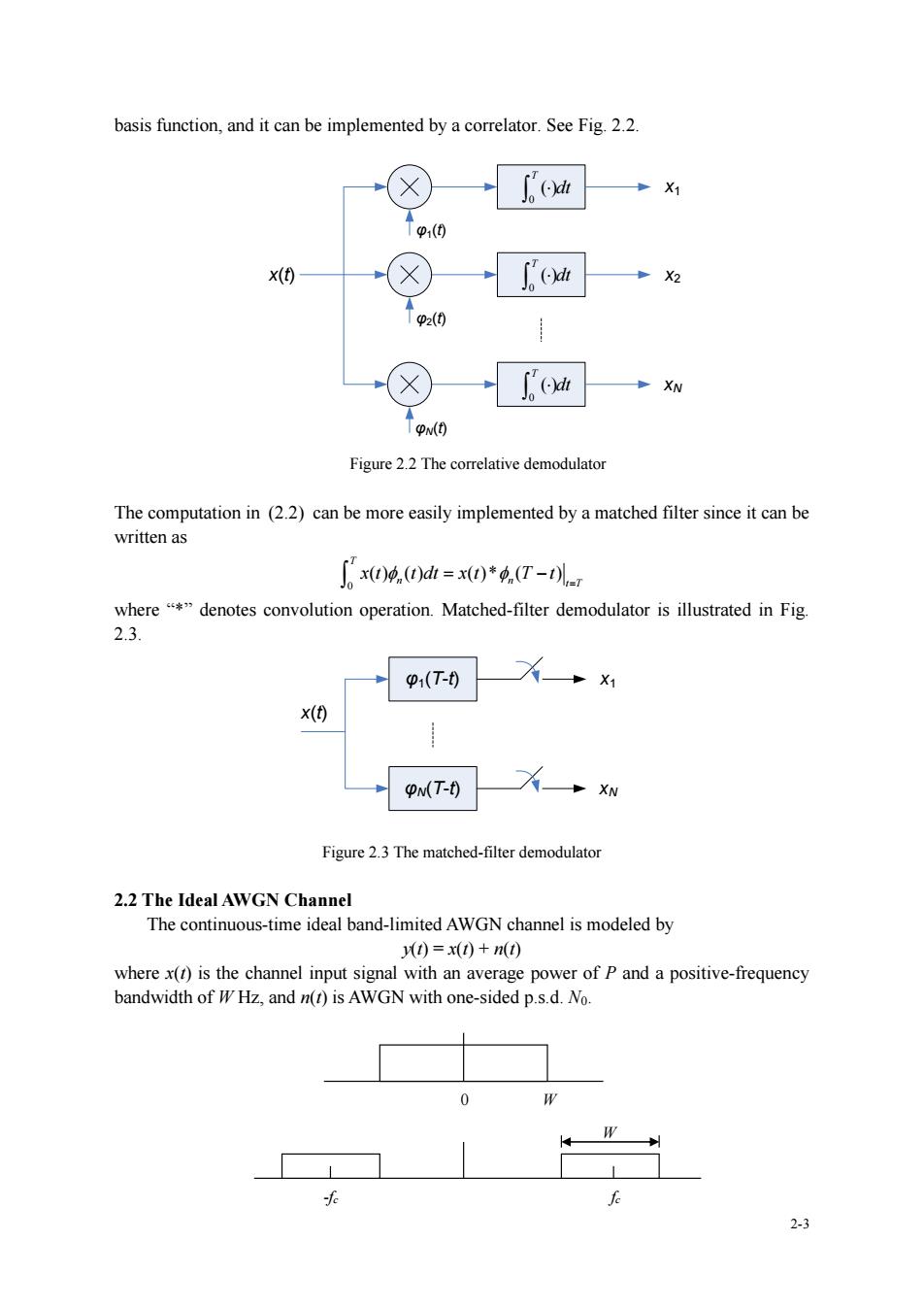
basis function,and it can be implemented by a correlator.See Fig.2.2. Tp1(0 x(t) fo Tp2(0 ox ↑p Figure 2.2 The correlative demodulator The computation in (2.2)can be more easily implemented by a matched filter since it can be a x0.0dh=xo)*.(T-儿 where"*"denotes convolution operation.Matched-filter demodulator is illustrated in Fig. 2.3. p1(T-0 pMT-用 Figure 2.3 The matched-filter demodulator 2.2 The Ideal AWGN Channel The continuous-time ideal band-limited AWGN channel is modeled by 0=x(0+n0 where()is the channel input signal with an average power of P and a positive-frequency bandwidth of W Hz,and n(t)is AWGN with one-sided p.s.d.No. 0
2-3 basis function, and it can be implemented by a correlator. See Fig. 2.2. 0 () T dt 0 () T dt 0 () T dt x1 x2 xN φ1(t) φ2(t) φN(t) x(t) Figure 2.2 The correlative demodulator The computation in (2.2) can be more easily implemented by a matched filter since it can be written as 0 ( ) ( ) ( )* ( ) T n n t T x t t dt x t T t = = − where “*” denotes convolution operation. Matched-filter demodulator is illustrated in Fig. 2.3. φ1(T-t) φN(T-t) x(t) x1 xN Figure 2.3 The matched-filter demodulator 2.2 The Ideal AWGN Channel The continuous-time ideal band-limited AWGN channel is modeled by y(t) = x(t) + n(t) where x(t) is the channel input signal with an average power of P and a positive-frequency bandwidth of W Hz, and n(t) is AWGN with one-sided p.s.d. N0. 0 W fc W -fc
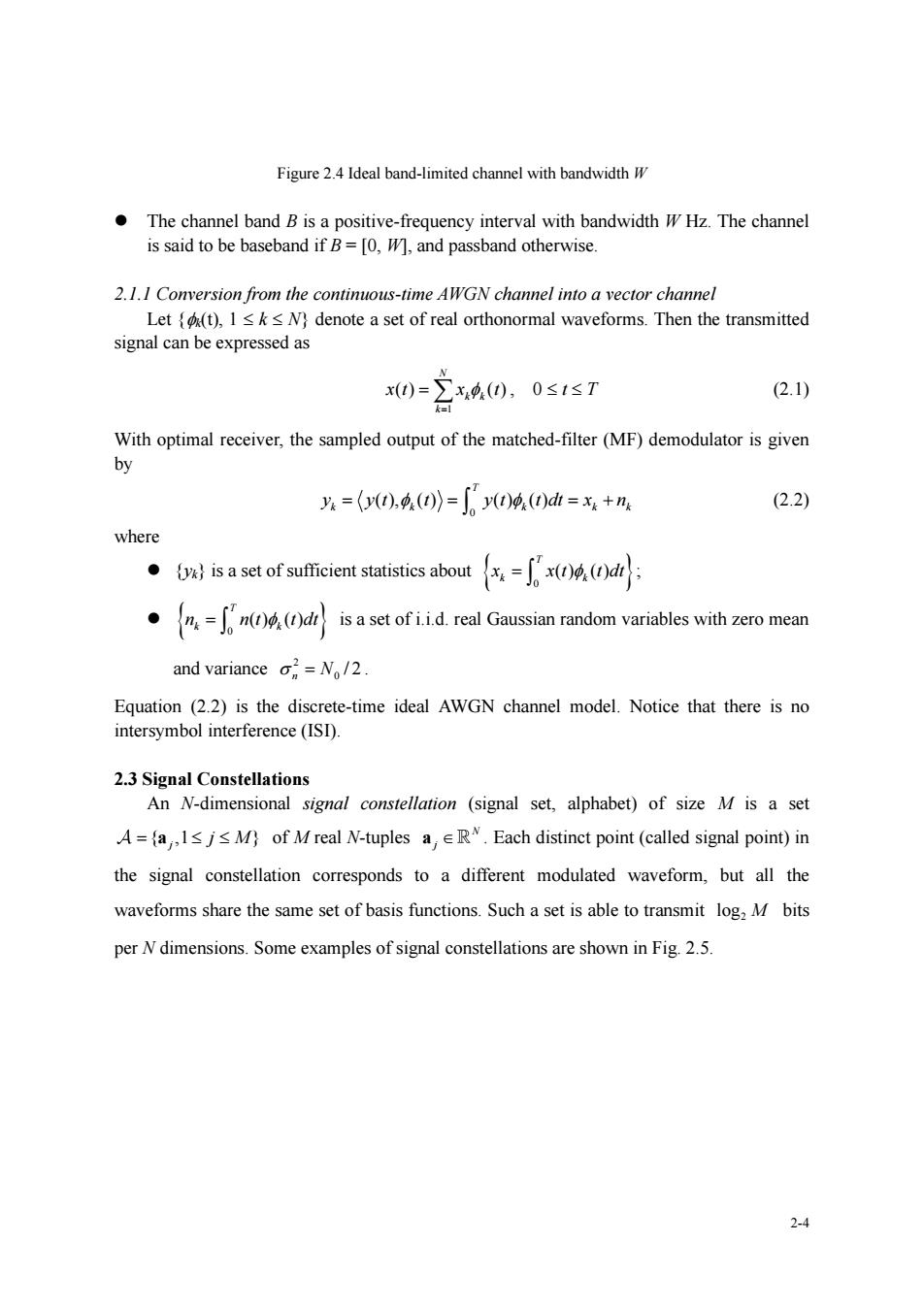
Figure 2.4 Ideal band-limited channel with bandwidth The channel band B is a positive-frequency interval with bandwidth W Hz.The channel is said to be baseband if B=[0,]and passband otherwise. 2.1.1 Conversion from the continous-time AWGN channel into a vector channel Lett),1sksN)denote a set of real orthonormal waveforms.Then the transmitted signal can be expressed as x(0=∑x4,0,0≤1≤T (2.1) With optimal receiver,the sampled output of the matched-filter(MF)demodulator is given by =(0),40》=∫y)40)d=x+n (2.2) where yis a set of sufficient statistics about(d (dr is a set of idreal Gaussian random variables with zero mean and variance =No/2 Equation (2.2)is the discrete-time ideal AWGN channel model.Notice that there is no intersymbol interference(ISI). 2.3 Signal Constellations An N-dimensional signal constellation (signal set.alphabet)of size M is a set A=ajsM)of Mreal N-tuples aR.Each distinct point(called signal point)in the signal constellation corresponds to a different modulated waveform,but all the waveforms share the same set of basis functions.Such a set is able to transmit log,M bits per Ndimensions.Some examples of signal constellations are shown in Fig.2.5
2-4 Figure 2.4 Ideal band-limited channel with bandwidth W ⚫ The channel band B is a positive-frequency interval with bandwidth W Hz. The channel is said to be baseband if B = [0, W], and passband otherwise. 2.1.1 Conversion from the continuous-time AWGN channel into a vector channel Let {k(t), 1 k N} denote a set of real orthonormal waveforms. Then the transmitted signal can be expressed as 1 ( ) ( ) N k k k x t x t = = , 0 t T (2.1) With optimal receiver, the sampled output of the matched-filter (MF) demodulator is given by 0 ( ), ( ) ( ) ( ) T k k k k k y y t t y t t dt x n = = = + (2.2) where ⚫ {yk} is a set of sufficient statistics about 0 ( ) ( ) T k k x x t t dt = ; ⚫ 0 ( ) ( ) T k k n n t t dt = is a set of i.i.d. real Gaussian random variables with zero mean and variance 2 0 /2 n = N . Equation (2.2) is the discrete-time ideal AWGN channel model. Notice that there is no intersymbol interference (ISI). 2.3 Signal Constellations An N-dimensional signal constellation (signal set, alphabet) of size M is a set { ,1 } j = a j M of M real N-tuples N a j . Each distinct point (called signal point) in the signal constellation corresponds to a different modulated waveform, but all the waveforms share the same set of basis functions. Such a set is able to transmit 2 log M bits per N dimensions. Some examples of signal constellations are shown in Fig. 2.5
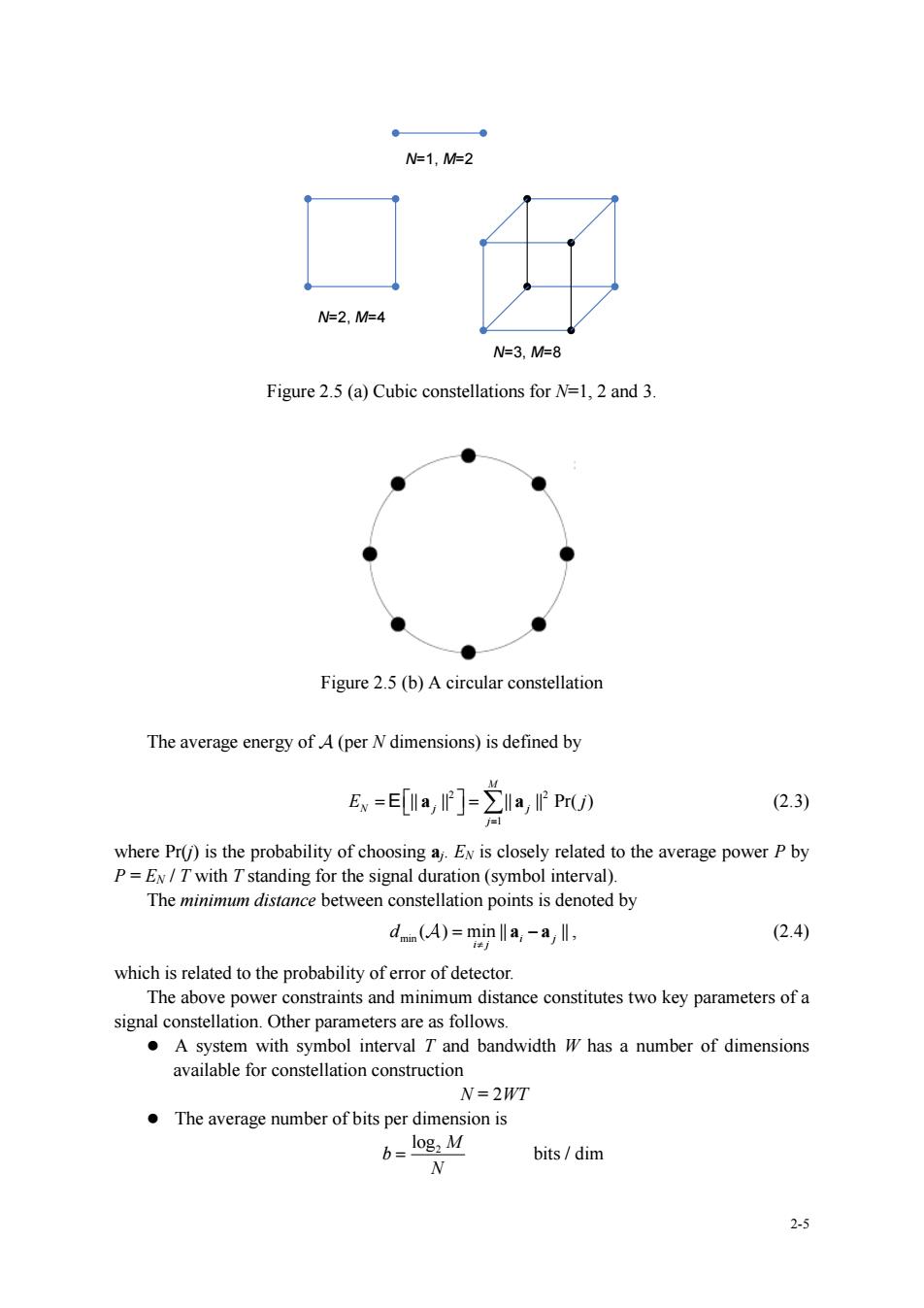
M1,M2 2,M4 W3,M=8 Figure 2.5(a)Cubic constellations for N=1,2 and 3. ●】 ● Figure 2.5(b)A circular constellation The average energy ofA(per N dimensions)is defined by E、=eIa,]-2Ia,rPmU) (2.3) where Pr()is the probability of choosinga EN is closely related to the average power P by P=E/T with Tstanding for the signal duration(symbol interval). The minimum distance between constellation points is denoted by dn(A)=min‖a,-a, (2.4) which is related to the probability of error of detector. The above power constraints and minimum distance constitutes two key parameters of a signal constellation.Other parameters are as follows. .A system with symbol interval T and bandwidth W has a number of dimensions avail ble N=2WT The average number of bits per dimension is b=log:M bits/dim 3
2-5 N=1, M=2 N=2, M=4 N=3, M=8 Figure 2.5 (a) Cubic constellations for N=1, 2 and 3. Figure 2.5 (b) A circular constellation The average energy of (per N dimensions) is defined by 2 2 1 || || || || Pr( ) M N j j j E j = = = E a a (2.3) where Pr(j) is the probability of choosing aj. EN is closely related to the average power P by P = EN / T with T standing for the signal duration (symbol interval). The minimum distance between constellation points is denoted by min ( ) min || || i j i j d = − a a , (2.4) which is related to the probability of error of detector. The above power constraints and minimum distance constitutes two key parameters of a signal constellation. Other parameters are as follows. ⚫ A system with symbol interval T and bandwidth W has a number of dimensions available for constellation construction N = 2WT ⚫ The average number of bits per dimension is 2 log M b N = bits / dim