0122229现代数字通信与编码理论 December 16,2008 XDU,Winter 2008 Lecture Notes Chapter 7 Coding and Modulation for Fading Channels physical channels may be characterized as time-varying fading channels.In this chapter,we will study communications over fading channels from an information-theoretic point of view. Many state-of-the-art coding and modulation schemes,including space-time codes,will be introduced. 7.1 Wireless Cha nne 1 Models 无线通信中,由于电波的反射、散射和绕射等,使得发射机和接收机之间有 在多条传播路径,并且每条路径的传播时延和衰耗因子都是时变的:在接收端,从不同 路径到达的信号分量叠加在一起,导致接收信号的强度随时间变化,我们通常用“衰落” 来描述这种现象。多径时变衰落是移动通信信道的主要特点。Many channel models arise or fading.Fi7.I depicts an overview of fading manifestations Fading channel manifestations Large-scale fading due to Small-scale fading due to motion over large areas small changes in position Variations about the mean Time spread Time-varying of the signal of the channel Frequence-selective fading ading ading Figure 7.1 7.1.1 Large-Scale Fading:Path loss and Shadowing Let s()=Rex()e be the transmitted signal,where x(t)x()e=R(e) is the complex baseband equivalent signal.In a fading environment,the magnitude of the received baseband waveform()can be expressed as |()Fa()R0=m)-()R()
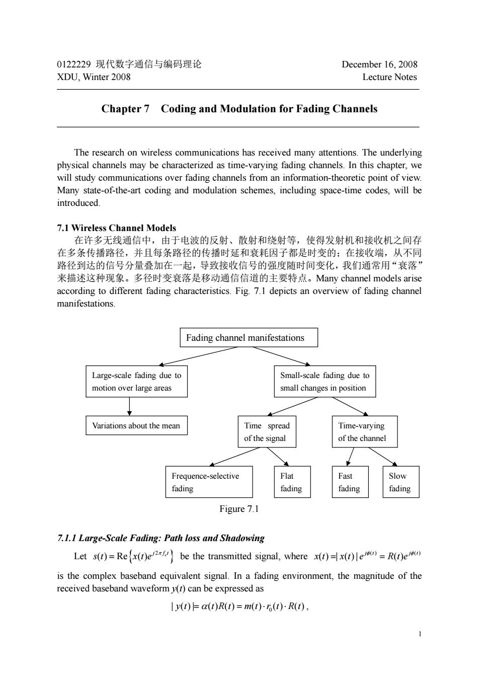
1 0122229 现代数字通信与编码理论 December 16, 2008 XDU, Winter 2008 Lecture Notes Chapter 7 Coding and Modulation for Fading Channels The research on wireless communications has received many attentions. The underlying physical channels may be characterized as time-varying fading channels. In this chapter, we will study communications over fading channels from an information-theoretic point of view. Many state-of-the-art coding and modulation schemes, including space-time codes, will be introduced. 7.1 Wireless Channel Models 在许多无线通信中,由于电波的反射、散射和绕射等,使得发射机和接收机之间存 在多条传播路径,并且每条路径的传播时延和衰耗因子都是时变的;在接收端,从不同 路径到达的信号分量叠加在一起,导致接收信号的强度随时间变化,我们通常用“衰落” 来描述这种现象。多径时变衰落是移动通信信道的主要特点。Many channel models arise according to different fading characteristics. Fig. 7.1 depicts an overview of fading channel manifestations. Figure 7.1 7.1.1 Large-Scale Fading: Path loss and Shadowing Let 2 ( ) Re ( ) c j ft st xte be the transmitted signal, where () () ( ) | ( )| ( ) jt jt x t xt e Rte is the complex baseband equivalent signal. In a fading environment, the magnitude of the received baseband waveform y(t) can be expressed as 0 | ( )| ( ) ( ) ( ) ( ) ( ) y t tRt mt r t Rt , Fading channel manifestations Large-scale fading due to motion over large areas Small-scale fading due to small changes in position Variations about the mean Time spread of the signal Time-varying of the channel Frequence-selective fading Flat fading Fast fading Slow fading
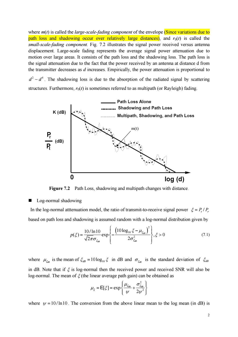
where m(t)is called the large-scale-fading component of the envelope(Since variations due to path loss and shadowing oc arge distances) and ro(t)is called the mall-scale-fadi ng component.Fig 72 illustrates the signal power received versus antenna displacement.Large-scale fading represents the average signal power attenuation due to motion over large areas.It consists of the path loss and the shadowing loss.The path loss is the signal attenuation due to the fact that the power received by an antenna at distance d from the transmitter decreases as d increases.Empirically,the power attenuation is proportional to d2-d.The shadowing loss is due to the absorption of the radiated signal by scattering structures.Furthermore,ro(r)is sometimes referred to as multipath(or Rayleigh)fading. Path Loss Alone .Shadowing and Path Loss K(dB) Multipath,Shadowing,and Path Loss m(0 公 (dB) 0 log (d) Figure 7.2 Path Loss,shadowing and multipath changes with distance. Log-normal shadowing In the log-normal atttenuation model,the ratio of transmit-to-receive signal power=P/P based on path loss and shadowing is assumed random with a log-normal distribution given by Pp(53=10/1n10 XD _(10g5-4l ,5>0 (7.1) where is the mean of=10log in dB and is the standard deviation of in dB.Note that if is log-normal then the received power and received SNR will also be log-normal.The mean of(the linear average path gain)can be btain where =10/In10.The conversion from the above linear mean to the log mean (in dB)is
2 where m(t) is called the large-scale-fading component of the envelope (Since variations due to path loss and shadowing occur over relatively large distances), and r0(t) is called the small-scale-fading component. Fig. 7.2 illustrates the signal power received versus antenna displacement. Large-scale fading represents the average signal power attenuation due to motion over large areas. It consists of the path loss and the shadowing loss. The path loss is the signal attenuation due to the fact that the power received by an antenna at distance d from the transmitter decreases as d increases. Empirically, the power attenuation is proportional to 2 4 d d . The shadowing loss is due to the absorption of the radiated signal by scattering structures. Furthermore, r0(t) is sometimes referred to as multipath (or Rayleigh) fading. Figure 7.2 Path Loss, shadowing and multipath changes with distance. Log-normal shadowing In the log-normal atttenuation model, the ratio of transmit-to-receive signal power / P P t r based on path loss and shadowing is assumed random with a log-normal distribution given by 2 10 2 10 / ln10 10log ( ) exp , 0 2 2 dB dB dB p (7.1) where 10 is the mean of 10log dB dB in dB and dB is the standard deviation of dB in dB. Note that if is log-normal then the received power and received SNR will also be log-normal. The mean of (the linear average path gain) can be obtained as dB dB 2 2 [ ] exp 2 E where 10 / ln10 . The conversion from the above linear mean to the log mean (in dB) is m(t)
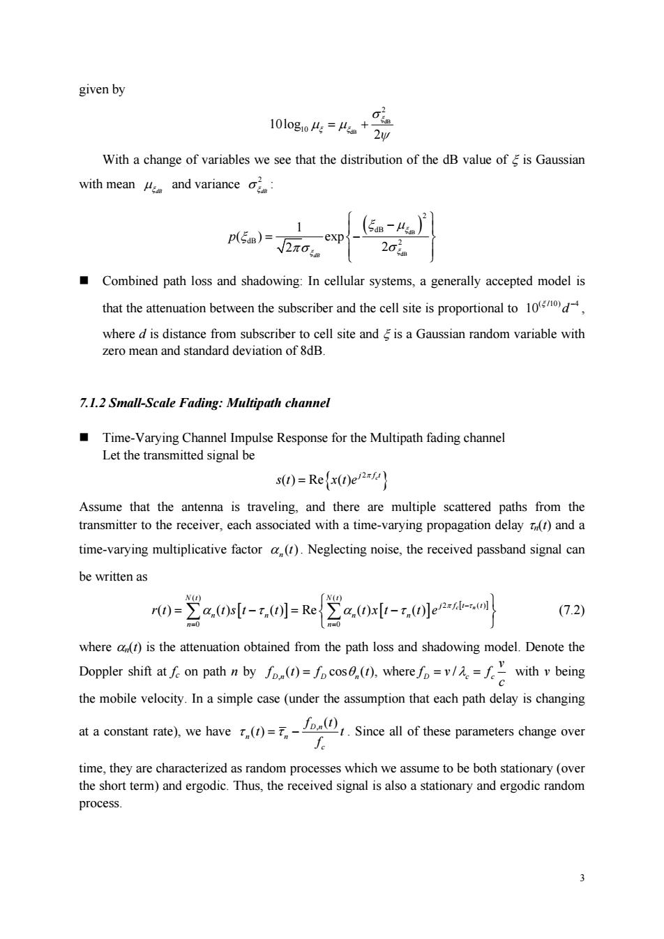
given by 0a从-儿+ With a change of variables we see that the distribution of the dB value of is Gaussian with mean and variance 1 pl5=2π0 -exp (5-4 Combined path loss and shadowing:In cellular systems,a generally accepted model is that the attenuation between the subscriber and the cell site is proportional to1 where d is distance from subscriber to cell site andis a Gaussian random variable with zero mean and standard deviation of 8dB. 7.1.2 Small-Scale Fading:Multipath channel Time-Varying Channel Impulse Response for the Multipath fading channel Let the transmitted signal be s(t)=Re(x(t)e Assume that the antenna is traveling.and there are multiple scattered paths from the transmitter to the receiver,each associated with a time-varying propagation delay()and a time-varying multiplicative factor (t).Neglecting noise,the received passband signal can be written as =。 ()st-r.(]-Re(-r.( (7.2) where)is the attenuation obtained from the path loss and shadowing model.Denote the Doppler shift at fe on path n by o ()=fcos,(t),where==with y being the mobile velocity.In a simple case(under the assumption that each path delay is changing ataconstant rate),we have(Since all of these parameters change over time,theyare characterized asrandom proces sses which we assume to be both stationary (ove the short term)and ergodic.Thus,the received signal is also a stationary and ergodic random process
3 given by dB dB 2 10 10log 2 With a change of variables we see that the distribution of the dB value of is Gaussian with mean dB and variance 2 dB : dB dB 2 dB dB 2 1 ( ) exp 2 2 dB p Combined path loss and shadowing: In cellular systems, a generally accepted model is that the attenuation between the subscriber and the cell site is proportional to ( /10) 4 10 d , where d is distance from subscriber to cell site and is a Gaussian random variable with zero mean and standard deviation of 8dB. 7.1.2 Small-Scale Fading: Multipath channel Time-Varying Channel Impulse Response for the Multipath fading channel Let the transmitted signal be 2 ( ) Re ( ) c j ft st xte Assume that the antenna is traveling, and there are multiple scattered paths from the transmitter to the receiver, each associated with a time-varying propagation delay n(t) and a time-varying multiplicative factor ( ) n t . Neglecting noise, the received passband signal can be written as () () 2 () 0 0 ( ) ( ) ( ) Re ( ) ( ) c n Nt Nt j ft t nn n n n n rt tst t txt t e (7.2) where n(t) is the attenuation obtained from the path loss and shadowing model. Denote the Doppler shift at fc on path n by , ( ) cos ( ), where / Dn D n D c c v f tf t fv f c with v being the mobile velocity. In a simple case (under the assumption that each path delay is changing at a constant rate), we have , ( ) ( ) D n n n c f t t t f . Since all of these parameters change over time, they are characterized as random processes which we assume to be both stationary (over the short term) and ergodic. Thus, the received signal is also a stationary and ergodic random process
ncoMpgoHeat Fig.7.4 Equation(7.2)can be rewritten as ro-Rea.0-. Since the channel may be subject to Doppler shifts,the recovered carrier,f at the receiver, might be different from the actual carrier Thus,the demodulated baseband signal is given by 0=∑a.0e2.ox-r.0)e2-d By letting()=()+,we can then rewrite the complex baseband equivalent signal as 0-2a0et-0叭 (7.3) Since a()depends on attenuation while()depends on delay and Doppler shift,we assume that these two random processes are independent.Equ.(7.3)描述了一个线性时变系 统的输入输出模型。 From(7.3),the equivalent lowpass time-varying impulse response(at timeto an impulse hc0-2a0ewar-0)-2A06(r-r0) (7.4) with B()(e This expression is quite nice.It says that the effect of mobile users. arbitrarily moving reflectors and absorbers,and all of the complexities of solving Maxwell's equations,finally reduce to an input/output relation between transmit and receive antennas which is simply represented as the impulse response of a linear time-varying channel filter. For the time-varying impulse responseh(),we can define a time-varying frequency
4 Fig. 7.4 Equation (7.2) can be rewritten as ( ) 2 () 2 0 ( ) Re ( ) ( ) cn c N t j f t j ft n n n rt te x t t e Since the channel may be subject to Doppler shifts, the recovered carrier, ˆ c f , at the receiver, might be different from the actual carrier fc. Thus, the demodulated baseband signal is given by ( ) ˆ 2 () 2 ( ) 0 () () () cn c c N t j f t j f ft n n n yt te xt t e By letting ˆ () 2 () 2 n cn c c t f t f ft , we can then rewrite the complex baseband equivalent signal as ( ) ( ) 0 () () () n N t j t n n n y t te xt t (7.3) Since ( ) n t depends on attenuation while ( ) n t depends on delay and Doppler shift, we assume that these two random processes are independent. Equ. (7.3) 描述了一个线性时变系 统的输入-输出模型。 From (7.3), the equivalent lowpass time-varying impulse response (at time t to an impulse transmitted at time t-) is given by () () ( ) 0 0 ( ,) () () () () n Nt Nt j t n n nn n n h t te t t t (7.4) with ( ) () () n j t n n t te . This expression is quite nice. It says that the effect of mobile users, arbitrarily moving reflectors and absorbers, and all of the complexities of solving Maxwell’s equations, finally reduce to an input/output relation between transmit and receive antennas which is simply represented as the impulse response of a linear time-varying channel filter. For the time-varying impulse response h(, t), we can define a time-varying frequency
response Hf:()=[hr.D)esdrB.(e One way of interpreting H(f.t)is to think of the system as a slowly varying function of t with a frequency response H(f r)at each fixed time t.Corresponding,h()can be thought of as the impulse response of the system at a fixed time t.This is a legitimate and useful way of thinking about multipath fading channels. as the time-scale at which the channel varies is typically much longer than the delay spread of the impulse response at a fixed time 7.1.3 Time and Frequency Coherence Wireless channels change both in time and frequency.The time coherence shows us how quickly the channel changes in time,and similarly,the frequency coherence shows how quickly it changes in frequency 7.1.3.I Delay spread and Coherence bandwidth Multipath delay spread The multipath delay spread of a channel h()is given by T.=max t,()-mint,() (7.5) For a single transmitted impulse,it represents the maximum excess delay,after which the multipath signal power falls below some threshold level relative to the strongest component. The minimum delay min()is often set to zero and the other multipath delays normalized root-mean-squared(rms)delay spread,defined as ,=F-可 where is the mean excess delay Multipath Intensity Profile The multipath intensity profile.also called the power delay profile,is defined as the autocorrelation E[h(,)h'(,)]=R()1-t)兰R(r) where=.It represents the average power associated with a given multipath delay. We can also characterize the time-varying multipath channel in the frequency domain. The autocorrelation of(is given by EH(f,)H'(f,t+△)]=R,(Af,△) where f=f-f.If we define R(Af)R(f.0),then it can be shown that
5 response ( ) 2 2 () 0 ( ;) ( ,) () n N t j f jft n n H f t h te d te One way of interpreting H(f; t) is to think of the system as a slowly varying function of t with a frequency response H(f; t) at each fixed time t. Corresponding, h(, t) can be thought of as the impulse response of the system at a fixed time t. This is a legitimate and useful way of thinking about multipath fading channels, as the time-scale at which the channel varies is typically much longer than the delay spread of the impulse response at a fixed time. 7.1.3 Time and Frequency Coherence Wireless channels change both in time and frequency. The time coherence shows us how quickly the channel changes in time, and similarly, the frequency coherence shows how quickly it changes in frequency. 7.1.3.1 Delay spread and Coherence bandwidth Multipath delay spread The multipath delay spread of a channel h(, t) is given by max ( ) min ( ) mn n n n T tt (7.5) For a single transmitted impulse, it represents the maximum excess delay, after which the multipath signal power falls below some threshold level relative to the strongest component. The minimum delay min ( ) n n t is often set to zero and the other multipath delays normalized with respect to this minimum delay. Another often used parameter to characterize the delay spread of the channel is the root-mean-squared (rms) delay spread, defined as 2 2 ( ) where is the mean excess delay. Multipath Intensity Profile The multipath intensity profile, also called the power delay profile, is defined as the autocorrelation * 1 2 1 12 ( ,) ( ,) ( ) ( ) () E h th t R R h h where 1 2 . It represents the average power associated with a given multipath delay. We can also characterize the time-varying multipath channel in the frequency domain. The autocorrelation of () is given by * 1 2 ( ,) ( , ) ( , ) E H f tH f t t R f t H where 2 1 f f f . If we define ( ) ( ,0) RH H fRf , then it can be shown that