西安电子科技大学：《现代数字通信与编码理论》课程教学资源（讲义）Chapter 08 Space-Time Coded-Modulation for Multiple Antenna Systems（for MIMO Channels）

0122229现代数字通信与编码理论 December 20,2008 XDU,Winter 2008 Lecture Notes Chapter 8 Space-Time Coded-Modulation for Multiple Antenna Systems (/for MIMO Channels) The advent of multiple-input-multiple-output (MIMO)space-time coded wireless systems has recently emerged as one of the most significant technical breakthroughs in modern communications.The research on MIMO systems,including the study of channel requirement of increasing bandwidth and transmit power). Note:The materials presented in Sections 8.3 and 8.6.3 are based largely on B.Vucetic's lecture notes. 8.1 Introduction An MIMO system is an arbitrary wireless communication system in which the transmitter as well as the receiver is equipped with multiple antenna elements.A core idea in MIMO systems is space-time signal processing in which time is complemented with the spatial dimension inherent in the use of multiple spatially distributed ntennas.MIMO effectively takes advantage of rand ng and multipath delay 图81给出了 read for ing transfer rate 有N根发送天线、M根接收天线的MMO系统框图。下图是采用不 同天线配置时的通信系统。 SISO MIMO TX/R< 乙RxWX SIMO MIMO-MU MISO Figure 8.0 Different antenna configurations in space-time systems

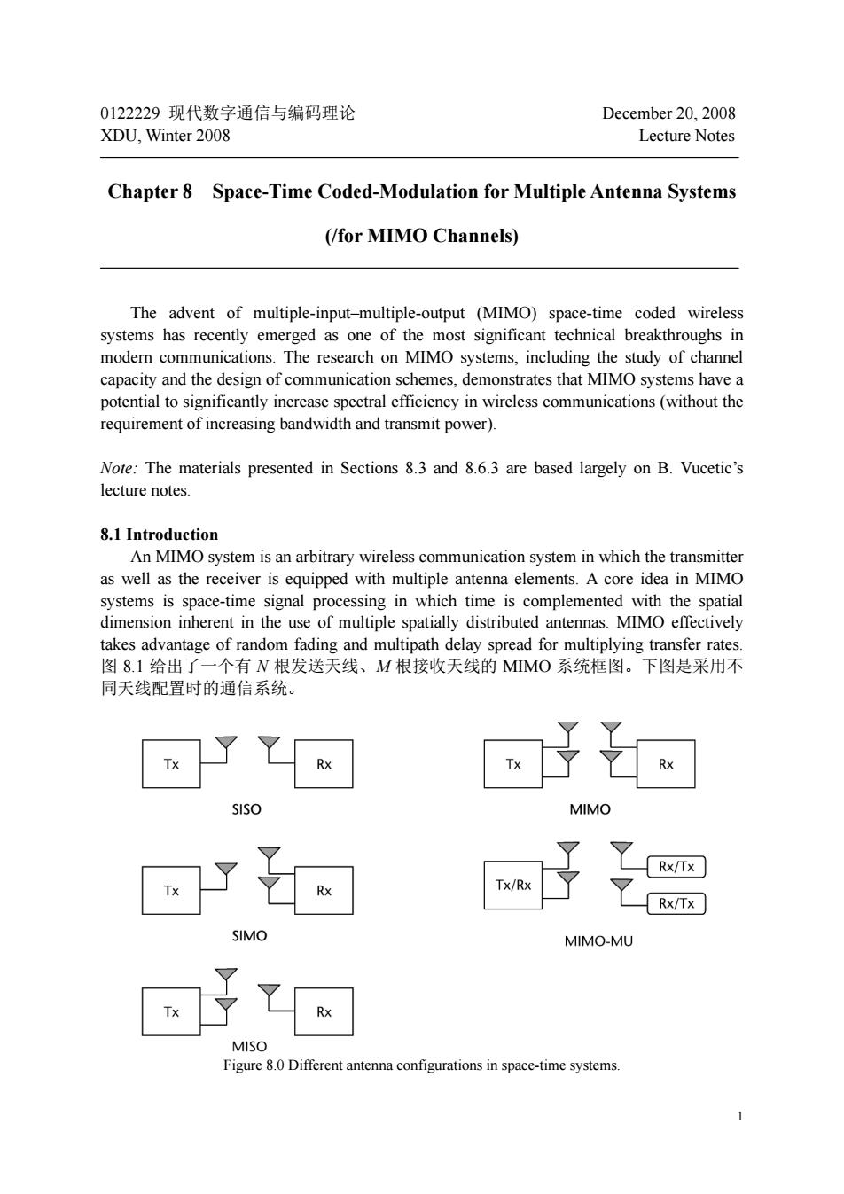
1 0122229 现代数字通信与编码理论 December 20, 2008 XDU, Winter 2008 Lecture Notes Chapter 8 Space-Time Coded-Modulation for Multiple Antenna Systems (/for MIMO Channels) The advent of multiple-input–multiple-output (MIMO) space-time coded wireless systems has recently emerged as one of the most significant technical breakthroughs in modern communications. The research on MIMO systems, including the study of channel capacity and the design of communication schemes, demonstrates that MIMO systems have a potential to significantly increase spectral efficiency in wireless communications (without the requirement of increasing bandwidth and transmit power). Note: The materials presented in Sections 8.3 and 8.6.3 are based largely on B. Vucetic’s lecture notes. 8.1 Introduction An MIMO system is an arbitrary wireless communication system in which the transmitter as well as the receiver is equipped with multiple antenna elements. A core idea in MIMO systems is space-time signal processing in which time is complemented with the spatial dimension inherent in the use of multiple spatially distributed antennas. MIMO effectively takes advantage of random fading and multipath delay spread for multiplying transfer rates. 图 8.1 给出了一个有 N 根发送天线、M 根接收天线的 MIMO 系统框图。下图是采用不 同天线配置时的通信系统。 Figure 8.0 Different antenna configurations in space-time systems

Winter、Foschini和Telatar的开创性工作证明，多天线阵技术可极大的提高系统信 道容量。若接收端可准确估计信道信息，并保证不同发射接收天线对之间的信道衰落 系数相互独立，则一个拥有N根发射天线和M根接收天线的MMO系统的信道容量将 随mi{MN线性增加。因此，信噪比、发射功率和信道带宽都相同时，多天线系统可 提供的信道容量是单天线系统的mi(M倍。在频率资源日益紧张的今天，多天线信 道容量理论无疑给解决高速无线通信问题开辟了一条新思路，基于此发展起来的信道编 码和信号处理技术正越来越受到人们的关注。 8.2 MIMO System Model nmunication system with N transmit and Mreceive The transmitted signal at time is represented by an Nx1 column vector xeC,and the received signal is represented by an Mx1 column vector yC(For simplicity,we ignore the time index).The discrete-time MIMOchannel can be described by y=Hx+n (8.1) where H is an MxN complex matrix describing the channel and the elementh,of H represents the channel gain from the transmit antenna to the receive antenna and n(0.N)is a zero-mean complex Gaussian noise vector whose components are ii.d.circularly symmetric complex Gaussian variables.The covariance matrix of the noise is given by KEnn]=N=,i.e.,each of Mreceive antennas has identical noise power of No(per complex dimension)(or,per real dimension).The total transmitted power is constrained to P,regardless of the number of transmit antennas N.It can be represented as Ex=E[xx]=E[Tr(x")]=TrEfxx=tr(K)sP. where K=Exxis the covariance matrix of the transmitted signal x.Furthermore,if the channel is unknown to the transmitter,we assume that the signals transmitted from individual antennas have equal powers of P/N.It means that K.= (8.2) The received signal covariance matrix,defined as K,=Eyy,is given by K,=Eyy"=HK,H"+NoI Denoting by P the average signal power at the output of each receive antenna,the average

2 Winter、Foschini 和 Telatar 的开创性工作证明，多天线阵技术可极大的提高系统信 道容量。若接收端可准确估计信道信息，并保证不同发射-接收天线对之间的信道衰落 系数相互独立，则一个拥有 N 根发射天线和 M 根接收天线的 MIMO 系统的信道容量将 随 min{M, N}线性增加。因此，信噪比、发射功率和信道带宽都相同时，多天线系统可 提供的信道容量是单天线系统的 min(M, N)倍。在频率资源日益紧张的今天，多天线信 道容量理论无疑给解决高速无线通信问题开辟了一条新思路，基于此发展起来的信道编 码和信号处理技术正越来越受到人们的关注。 8.2 MIMO System Model Consider a single-user MIMO communication system with N transmit and M receive antennas. (It will be called a (N, M) system.) The system block diagram is shown in Fig.8.1. The transmitted signal at time t is represented by an N1 column vector N x  , and the received signal is represented by an M1 column vector M y  (For simplicity, we ignore the time index). The discrete-time MIMO channel can be described by y  Hx n  (8.1) where H is an MN complex matrix describing the channel and the element ij h of H represents the channel gain from the transmit antenna j to the receive antenna i; and   0 , n 0I   N M is a zero-mean complex Gaussian noise vector whose components are i.i.d. circularly symmetric complex Gaussian variables. The covariance matrix of the noise is given by 2 0 [] 2 H K nn I I n MM   E N  , i.e., each of M receive antennas has identical noise power of N0 (per complex dimension) (or,  2 per real dimension). The total transmitted power is constrained to P, regardless of the number of transmit antennas N. It can be represented as   2 || || ( ) tr( ) HHH Tr Tr P x             E EE E K x x x xx xx , where = H x   K xx   E is the covariance matrix of the transmitted signal x. Furthermore, if the channel is unknown to the transmitter, we assume that the signals transmitted from individual antennas have equal powers of P/N. It means that x N P N K I  (8.2) The received signal covariance matrix, defined as = H y   K   E yy , is given by 0 H H y xM    N K   E yy HK H I Denoting by Pr the average signal power at the output of each receive antenna, the average

SNR at each receive antenna is given by SNR-7-N. which is independent of N.The total received signal power can be expressed asTr(K) h 7 h 2 空时 ④ 空时 发送 接收 ny Fig.8.1 An MIMO wireless system model We will consider several possible scenarios for the matrix H: 1.H is deterministic 2.H is a random matrix.Its entries are selected according a probability distribution at the beginning of each symbol interval T and are kept constant during one symbol interval.In each of the cha corresp ding to an inc dependent ealization of H. ing channel. 3.H is a random matrix.Its entries change randomly and are kept constant during a fixed number of symbol intervals,much shorter than a transmission block.Such a channel is called a block fading channel. 4.H is a random matrix but is fixed at the start of a transmission block and kept constant Such a channel is called a slow or quasi-static fading channel For normalization purposes,we assume that the received power for each of M receive branches is equal to the total transmitted power.Thus,in the case when H is deterministic,we have F-N.n.2. When H is random,we will assume that its entries are i.i.d.zero-mean complex Gaussian with variance per dimension.This scase is usually referred to as a rich scattering environmen.The normalization constraint for the elements of H is given by 2E[h门=N,m=l2M

3 SNR at each receive antenna is given by 0 Pr N SNR    which is independent of N. The total received signal power can be expressed asTr( ) K y .    Fig. 8.1 An MIMO wireless system model We will consider several possible scenarios for the matrix H: 1. H is deterministic. 2. H is a random matrix. Its entries are selected according a probability distribution at the beginning of each symbol interval T and are kept constant during one symbol interval. In other words, each use of the channel corresponding to an independent realization of H. Such a channel is called a fast (or independent) fading channel. 3. H is a random matrix. Its entries change randomly and are kept constant during a fixed number of symbol intervals, much shorter than a transmission block. Such a channel is called a block fading channel. 4. H is a random matrix but is fixed at the start of a transmission block and kept constant during a transmission block. Such a channel is called a slow or quasi-static fading channel. For normalization purposes, we assume that the received power for each of M receive branches is equal to the total transmitted power. Thus, in the case when H is deterministic, we have 2 1 | | , 1,2,., N mn n h Nm M     When H is random, we will assume that its entries are i.i.d. zero-mean complex Gaussian variables, each with variance 1/2 per dimension. This case is usually referred to as a rich scattering environment. The normalization constraint for the elements of H is given by 2 1 | | , 1,2,., N mn n h Nm M         E

With the normalization constraint,the total received signal power per antenna is equal to the total transmitted power,and the average SNR at any receive antenna isy=P/N. In all cases,we will assume that the channel matrix is known to the receiver(ie.,perfect CSIR),equivalently,the channel output consists of the pair(y,H),and the distribution of H is known at the transmitter.In most situations,the realization of H(CSI)is assumed to be not known at the transmitter. 8.3 Fundamental Capacity Limits of MIMO Channels Consider the case of deterministic H.The channel matrix H is assumed to be constant at all time and known to the receiver.The relation of(8.1)indicates a vector Gaussian channel. The Shannon capacity is defined as the maximum data rate that can be transmitted over the mation C(H)= mZ,田=m8xZx+Zxy田 =max Z(x;y H)=max [H(yH)-H(ylx,H)] (8.3) where p(x)is the probability distribution of the vector x,H(y|H)and H(yx,H)are the differential entropy and the conditional differential entropy of the vector y,respectively.Since the vectors x and n are independent,we have Hylx,H)=H(n)=log2(det(πeW。Iy) which has fixed value and is independent of the channel input.Thus,maximizing the mutual information I(x:y|H)is equivalent to maximize H(yH).From (8.1),the covariance matrix ofy is K,=E["]=HKH"+N。Iw Among all vectors y with a given covariance matrix K.the differential entropy H(y)is maximized when y is a zero-mean circularly symmetric complex Gaussian (ZMCSCG) random vector [Telatar9].This implies that the inputx must also be ZMCSCG and therefore this is the optimal distribution onx.This yields the entropy H(yH)given by H(y|H)=log,(det(eK,)) The mutual information then reduces to Z(x:y|H)=H(y|H)-H(n) log,det (8.4)

4 With the normalization constraint, the total received signal power per antenna is equal to the total transmitted power, and the average SNR at any receive antenna is 0   P N/ . In all cases, we will assume that the channel matrix is known to the receiver (i.e., perfect CSIR), equivalently, the channel output consists of the pair (y, H), and the distribution of H is known at the transmitter. In most situations, the realization of H (CSI) is assumed to be not known at the transmitter. 8.3 Fundamental Capacity Limits of MIMO Channels Consider the case of deterministic H. The channel matrix H is assumed to be constant at all time and known to the receiver. The relation of (8.1) indicates a vector Gaussian channel. The Shannon capacity is defined as the maximum data rate that can be transmitted over the channel with arbitrarily small error probability. It is given in terms of the mutual information between vectors x and y as 2 ( ): [|| || ] ( ) ( ) max ( ; , ) max ( ; ) ( ; | ) p P p x C    x x H x   y H xH x y H E   () () max ( ; | ) max ( | ) ( | , ) px px     x y H y H y x H (8.3) where p(x) is the probability distribution of the vector x,   ( | ) and ( | , ) y H y x H are the differential entropy and the conditional differential entropy of the vector y, respectively. Since the vectors x and n are independent, we have   ( | , ) ( ) log det( ) y xH n I   2 0  eN M  which has fixed value and is independent of the channel input. Thus, maximizing the mutual information ( ; | )  x y H is equivalent to maximize ( | )  y H . From (8.1), the covariance matrix of y is = 0 H H y xM     N K   E K yy HH I Among all vectors y with a given covariance matrix Ky, the differential entropy ( )  y is maximized when y is a zero-mean circularly symmetric complex Gaussian (ZMCSCG) random vector [Telatar99]. This implies that the input x must also be ZMCSCG, and therefore this is the optimal distribution on x. This yields the entropy ( | )  y H given by ( | ) log det( ) y H  2  eK y  The mutual information then reduces to   (; | ) ( | ) () x y H   y H n 2 0 1 log det H M x N               I HH K (8.4)

where we have used the fact that det(AB)=det(A)det(B)and det(A-)=[det(A)].And the MIMO capacity is given by maximizing the mutual information (8.4)over all input covariance matrces K,satistying the power constraint c器，ogda+Kr》 bits per channel use (8.5) -腮a+之kr列 where the last equality follows from the fact that det(I+AB)=det(I+BA)for matrices A(mxm)andB(n×m) Clearly,the optimization relative to K.will depend on whether or not H is known at the transmitter.We now discuss this maximizing under different assumptions about transmitter CSI by decomposing the vector channel into a set of parallel,independent scalar Gaussian sub-channels. 8.3.1 Parallel Decomposition of the MIMO Channel By the singular value decomposition(SVD)theorem,any MxN matrix HECN can be written as H=UAVI (8.6) where A is an MN non-negative real and diagonal matrix.U and V are MxM and NxN unitary matrices,respectively.That is.UU=I and VV=where the superseript entries of A are the non-negat e columns of U are the eigenvectors of HH and the columns of Vare the eigenvectors of HH. Denote by Athe eigenvalues of HH",which are defined by HH"z=z,z0 (87) mber of no cannot exceed the number of columns or rows of H,rsm=min(M,N).If H is full rank, which is sometimes referred to as a rich scattering environment,thenr=m.Equation (8.7) can be rewritten as (2L.-W)z=0,z0 (8.8) where W is the Wishart matrix defined to be 5

5 where we have used the fact that det( ) det( )det( ) AB A B  and   1 1 det( ) det( )   A A  . And the MIMO capacity is given by maximizing the mutual information (8.4) over all input covariance matrces Kx satisfying the power constraint: 2 :( ) 0 1 ( ) max log det x x H M x Tr P C  N               H I HH K K K bits per channel use (8.5) 2 :( ) 0 1 max log det x x H N x Tr P N               I HH K K K where the last equality follows from the fact that det det I AB I BA m n      for matrices A B ( ) and ( ) mn nm   . Clearly, the optimization relative to Kx will depend on whether or not H is known at the transmitter. We now discuss this maximizing under different assumptions about transmitter CSI by decomposing the vector channel into a set of parallel, independent scalar Gaussian sub-channels. 8.3.1 Parallel Decomposition of the MIMO Channel By the singular value decomposition (SVD) theorem, any MN matrix M N H can be written as H H U ΛV (8.6) where  is an MN non-negative real and diagonal matrix, U and V are MM and NN unitary matrices, respectively. That is, and H H UU I VV I  M  N , where the superscript “H” stands for the Hermitian transpose (or complex conjugate transpose). In fact, the diagonal entries of  are the non-negative square roots of the eigenvalues of matrix HHH, the columns of U are the eigenvectors of HHH and the columns of V are the eigenvectors of HHH. Denote by  the eigenvalues of HHH, which are defined by H HH z z   , z0 (8.7) where z is an M1 eigenvector corresponding to . The number of non-zero eigenvalues of matrix HHH is equal to the rank of H. Let r be the rank of the matrix H. Since the rank of H cannot exceed the number of columns or rows of H, min( , ) r m MN   . If H is full rank, which is sometimes referred to as a rich scattering environment, then r = m. Equation (8.7) can be rewritten as ( ) 0, I Wz m   z0 (8.8) where W is the Wishart matrix defined to be