0122229现代数字通信与编码理论 October 1,2010 XDU,Fall 2010 Lecture Notes Chapter 3 Performance Bounds of Coded Communication Systems since the error performance of coded communication systems rarely admits exact express analytical uppe and lower bounds serve s a useful theoretical a nd engineering tool for assessing performance and for gaining insight into the effect of the main system parameters.As specific good codes are hard to identify,the performance of ensembles of codes is usually considered. In this chapter we will study the bounding techniques used for performance analysis of coded communication system s with em nphasis on the understanding of Bhattacharyya bound and Gallager bound. n particular.Gal ger bound provides a better upper bound on the ML decoding error probability for a specific code and ensemble of random/structured codes. (Gallager bound was introduced in [Gallager65]as an efficient tool to determine the error exponents of the ensemble of random codes.providing informative results up to the ultimate acity limit We will also show that it is possible to approach capacity on arb itrary DMCs with coding It should be pointed out that although maximum-likelihood (ML)decoding is in genera prohibitively complex for long codes,the derivation of upper and lower bounds on the ML decoding error probability is of interest,providing an ultimate indication of the system performance. Note:The materials presented in Sections 3.3 through 3.7 are based largely on Massey's lecture notes 3.1 Mathematical Preliminaries 3 1 I Basic inegualities Markov Inequality The Markov inequality states that if a non-negative random variable Y has a mean E[Y]. then the probability that the outcome exceeds any given number satisfies PW≥)s] (3.1) Chebyshev Inequality Let Z be an arbitrary random variable with finite mean E[Z]and finite variance o. Define Y as the non-negative random variable Y=(Z-E[Z]).The E[Y]=2 Applying (3.1). P((Z-EZ 1 心
3-1 0122229 现代数字通信与编码理论 October 1, 2010 XDU, Fall 2010 Lecture Notes Chapter 3 Performance Bounds of Coded Communication Systems Since the error performance of coded communication systems rarely admits exact expressions, tight analytical upper and lower bounds serve as a useful theoretical and engineering tool for assessing performance and for gaining insight into the effect of the main system parameters. As specific good codes are hard to identify, the performance of ensembles of codes is usually considered. In this chapter we will study the bounding techniques used for performance analysis of coded communication systems, with emphasis on the understanding of Bhattacharyya bound and Gallager bound. In particular, Gallager bound provides a better upper bound on the ML decoding error probability for a specific code and ensemble of random/structured codes. (Gallager bound was introduced in [Gallager65] as an efficient tool to determine the error exponents of the ensemble of random codes, providing informative results up to the ultimate capacity limit.) We will also show that it is possible to approach capacity on arbitrary DMCs with coding. It should be pointed out that although maximum-likelihood (ML) decoding is in general prohibitively complex for long codes, the derivation of upper and lower bounds on the ML decoding error probability is of interest, providing an ultimate indication of the system performance. Note: The materials presented in Sections 3.3 through 3.7 are based largely on Massey’s lecture notes. 3.1 Mathematical Preliminaries 3.1.1 Basic Inequalities Markov Inequality The Markov inequality states that if a non-negative random variable Y has a mean E[Y], then the probability that the outcome exceeds any given number satisfies [ ] ( ) Y PY y y ≥ ≤ E (3.1) Chebyshev Inequality Let Z be an arbitrary random variable with finite mean E[Z] and finite variance 2 σ Z . Define Y as the non-negative random variable 2 YZ Z = − ( [ ]) E . The E[Y] = 2 σ Z . Applying (3.1), { } 2 2 ( [ ]) Z PZ Z y y σ − ≥≤ E
Replacing y with(for any )this becomes the well-known Chebyshev inequality P(lZ-EZI)s (3.2) Chernoff Bound(or Exponential bound) Let Y=exp(sZ)for some arbitrary random variable Z that has a moment generating function gz(s)=E[exp(sZ)]over some open interval of real values ofs including s=0. Then,fors in that interval,(3.1)becomes P(exp(sz)() Lettingy=exp(s)for some constant we have P(Z≥6)≤eEe21,fors≥0 (3.3) P(Z≤6)≤ewEe2l,fors≤0 The bounds can be optimized overs to get the strongest bound. Jensen's Inequality If fis a convex-function and is a random variable,then ELf(XI≥(E[X]) (3.4) Moreover,iff is strictly convex,then equality in (3.4)implies that with probability 1,i.e.is a constant. The Union n Bound For sets Aand B,we have P(AUB)=P(A)+P(B)-P(AB) Since P(AnB)≥0, P(AUB)≤P(A)+P(B) 3.2 Block Coding Principles In the following discussions,we will restrict our attention to block encoders and decoders Consider a discrete memoryless channel (DMC)with input alphabet A= and output alphabet A.=(bbb.A block code of length N with Mcodewords for such a channel is a list ().each item of which is an N-tuple of elements from Ax.See Fig.3.1.We will denote the incoming message index by Z.whose possible values are integers from I through M=2,where L is the length of input binary data sequence.We assume that when the information sequence corresponding to integer m enters the encoder,the codeword 3-2
3-2 Replacing y with ε 2 (for any ε>0), this becomes the well-known Chebyshev inequality { } 2 2 | [ ]| Z PZ Z σ ε ε − ≥≤ E (3.2) Chernoff Bound (or Exponential bound) Let Y = exp(sZ) for some arbitrary random variable Z that has a moment generating function ( ) [exp( )] Z g s sZ = E over some open interval of real values of s including s=0. Then, for s in that interval, (3.1) becomes { } ( ) exp( ) Z g s P sZ y y ≥ ≤ Letting y = exp(sδ) for some constant δ, we have ( ) [ ], for 0 ( ) [ ], for 0 s sZ s sZ PZ e e s PZ e e s δ δ δ δ − − ≥≤ ≥ ≤ ≤ ≤ E E (3.3) The bounds can be optimized over s to get the strongest bound. Jensen’s Inequality If f is a convex-∪ function and X is a random variable, then E E [ ( )] ( [ ]) f X fX ≥ (3.4) Moreover, if f is strictly convex, then equality in (3.4) implies that X=E[X] with probability 1, i.e., X is a constant. The Union Bound For sets A and B, we have PA B PA PB PA B ( ) () () ( ) ∪= + − ∩ Since ( ) 0 PA B ∩ ≥ , PA B PA PB ( ) () () ∪≤ + 3.2 Block Coding Principles In the following discussions, we will restrict our attention to block encoders and decoders. Consider a discrete memoryless channel (DMC) with input alphabet 1 2 { , ,., } X K A = aa a and output alphabet 1 2 { , ,., } Y J A = bb b . A block code of length N with M codewords for such a channel is a list 1 2 ( , ,., ) M xx x , each item of which is an N-tuple of elements from AX. See Fig. 3.1. We will denote the incoming message index by Z, whose possible values are integers from 1 through M = 2L , where L is the length of input binary data sequence. We assume that when the information sequence corresponding to integer m enters the encoder, the codeword
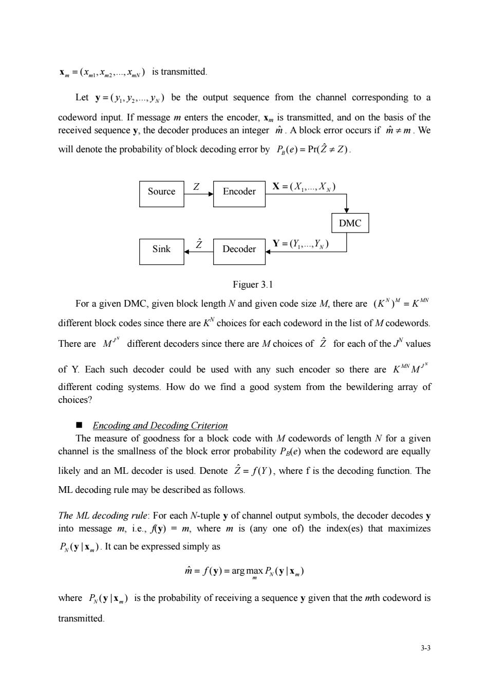
=(is transmitted. Let y=(.)be the output sequence from the channel corresponding to a codeword input.If message m enters the encoder,is transmitted,and on the basis of the received sequence y,the decoder produces an integer A block error occurs ifm.We will denote the probability of block decoding error by P(e)=Pr(Z). Source Encoder=() DMC Sink Decoder Y=(Y.Yy) Figuer 3.1 For a given DMC,given block length Nand given code size M.there are (K)=K different block codes since there are Kchoices for each codeword in the list of Mcodewords. There areM different decoders since there are Mchoices of for each of thevalues of Y.Each such decoder could be used with any such encoder so there are different coding systems.How do we find a good system from the bewildering array of choices? Encoding and Decoding Criterion measure Tg000 a block code with M codewords of length N for a give channel is the smallness of the block error probability Pa(e)when the codeword are equally likely and an ML decoder is used.Denote Z=f(Y),where f is the decoding function.The ML decoding rule may be described as follows. The ML decoding rule:For each N-tuple y of channel output symbols,the decoder decodesy into message m,i.e.,fy)=m,where m is (any one of)the index(es)that maximizes P(y).It can be expressed simply as =f(y)=argmax P(ylx) where P(yx)is the probability of receiving a sequence y given that the mth codeword is transmitted. 3.3
3-3 1 2 ( , ,., ) m m m mN x = x x x is transmitted. Let 1 2 ( , ,., ) N y = y y y be the output sequence from the channel corresponding to a codeword input. If message m enters the encoder, xm is transmitted, and on the basis of the received sequence y, the decoder produces an integer mˆ . A block error occurs if m m ˆ ≠ . We will denote the probability of block decoding error by ˆ ( ) Pr( ) Pe Z Z B = ≠ . Figuer 3.1 For a given DMC, given block length N and given code size M, there are ( ) N M MN K K= different block codes since there are KN choices for each codeword in the list of M codewords. There are N J M different decoders since there are M choices of Zˆ for each of the J N values of Y. Each such decoder could be used with any such encoder so there are N MN J K M different coding systems. How do we find a good system from the bewildering array of choices? Encoding and Decoding Criterion The measure of goodness for a block code with M codewords of length N for a given channel is the smallness of the block error probability PB(e) when the codeword are equally likely and an ML decoder is used. Denote ˆ Z = f Y( ), where f is the decoding function. The ML decoding rule may be described as follows. The ML decoding rule: For each N-tuple y of channel output symbols, the decoder decodes y into message m, i.e., f(y) = m, where m is (any one of) the index(es) that maximizes (| ) PN m y x . It can be expressed simply as ˆ ( ) arg max ( | ) N m m mf P = = y y x where ( | ) PN m y x is the probability of receiving a sequence y given that the mth codeword is transmitted. Source Encoder DMC Sink Decoder 1 ( ,., ) Z X = X X N 1 ( ,., ) Y = Y YN Zˆ

In the case of a DMC used without feedback,this becomes m=f)=arg max·P0.x) 3.3 Codes with Two Codewords-the Bhattacharyya Bound We will denote the set of received sequences decoded into message.e. D.=yeA*If(y)=m which is called the decision region for message m.Since the output sequence y is decoded (/mapped)to exactly one message,D's form a collection of disjoint sets whose union isA ie. [DnD,=g,for all i≠j UD- Thus,the probability of decoding eror,when messagemis sent,is defined as P(elm)=Pr(2+ZIZ=m)=Pr(yDx) =l-Pry∈DIxn)=∑Pylx) (3.5) VeD. The overall probability of decoding error,if the message have a priori distribution Pr(m),is then given by P.()-p(m)F.(em) (3.6) Equations(3.5)and (3.6)apply to any block code and any channel.In particular,the case is simple whenM2.In this case,the error probability,when message 2 is transmitted,is BeI2-gB) (3.7) We observe that, for yeDi,P.(yx )2 P(yx) for ML decoding.It also implies that P(yx(y),<s<1,and hence that P(ylx)s P(yx2)P(ylx)' (3.8) Substituting (3.8)into (3.7)and lettings=1/2,we have P.(e12)s>P(ylx)P(ylx2) (3.9) Similarly, (3.10) 34
3-4 In the case of a DMC used without feedback, this becomes , 1 ˆ ( ) arg max ( | ) N n mn m n m f Py x = = = y ∏ 3.3 Codes with Two Codewords – the Bhattacharyya Bound We will denote the set of received sequences decoded into message m as Dm; i.e., { | () } N m Y D A =∈ = y y f m which is called the decision region for message m. Since the output sequence y is decoded (/mapped) to exactly one message, Dm’s form a collection of disjoint sets whose union is N AY ; i.e., , for all i j N i Y i ⎧ ∩ = ≠ φ i j ⎪ ⎨ = ⎪⎩ ∪ D D D A Thus, the probability of decoding error, when message m is sent, is defined as ˆ ( | ) Pr( | ) Pr( | ) P em Z ZZ m B mm ≡ ≠ == ∉y x D 1 Pr( | ) ( | ) m mm N m P ∉ =− ∈ = ∑ y y x y x D D (3.5) The overall probability of decoding error, if the message have a priori distribution Pr(m), is then given by 1 ( ) Pr( ) ( | ) M B B m P e mP e m = = ∑ (3.6) Equations (3.5) and (3.6) apply to any block code and any channel. In particular, the case is simple when M = 2. In this case, the error probability, when message 2 is transmitted, is 1 2 ( | 2) ( | ) Pe P B N ∈ = ∑ y y x D (3.7) We observe that, for y∈D1, 1 2 (| ) (| ) P P N N y x ≥ y x for ML decoding. It also implies that 1 2 (| ) (| ) s s P P N N y x ≥ y x , 0 < s < 1, and hence that 1 2 21 (| ) (| ) (| ) s s PPP NNN − y x ≤ y x y x (3.8) Substituting (3.8) into (3.7) and letting s=1/2, we have 1 1 2 ( | 2) ( | ) ( | ) Pe P P B NN ∈ ≤ ∑ y y x y x D (3.9) Similarly, 2 1 2 ( |1) ( | ) ( | ) Pe P P B NN ∈ ≤ ∑ y y x y x D (3.10)
Combining (3.9)and (3.10),we obtain P.(eIl)+P.(el2)≤∑P,(yIx)R(yIx2) (3.11) Notice that the summation is now over all y and hence is considerably easier to evaluate. Because Pa(el)and P(e2)are non-negative,the R.H.S.of (3.11)is an upper bound on each of these conditional error probabilities.Thus,we have P.(elm)sP(ylx)P(ylx2).m 1.2 (3.12) For the special case ofa DMC,it simplifies to P(em)≤Π∑√(yx)P(y川xa),m=L,2 (3.13) where we have written the dummy variable of summation asyrather than y The bound in (3.12)and (3.13)are known as the Bhattacharyya bound on error probability. Defining da=-log P(ylx)P(ylx2) (3.14) which we will call the Bhattacharyya distance between the two channel input sequences,we can rewrite (3.12)as Pa(elm)≤2,m=l,2 In the special case of a binary-input DMC and the repetition code of length N.(3.13)becomes P.(elm)s∑√PylO)PyI西,m=1,2 which can be written as Pa(elm)≤2o,m=L,2 where Da=-log∑P(y10)P(y) Note:The bound in (3.12)can also be interpreted as a Chernoff bound as follows. seE exps-logw1s2」 P(ylx.) -.(yx) hems.msy 35
3-5 Combining (3.9) and (3.10), we obtain 1 2 ( |1) ( | 2) ( | ) ( | ) Pe Pe P P B B NN + ≤ ∑ y y x y x (3.11) Notice that the summation is now over all y and hence is considerably easier to evaluate. Because PB(e|1) and PB(e|2) are non-negative, the R.H.S. of (3.11) is an upper bound on each of these conditional error probabilities. Thus, we have 1 2 (| ) (| ) (| ) P em P P B NN ≤ ∑ y y x y x , m = 1, 2 (3.12) For the special case of a DMC, it simplifies to 1 2 1 (| ) ( | )( | ) N B nn n y P em Py x Py x = ≤ ∏∑ , m = 1, 2 (3.13) where we have written the dummy variable of summation as y rather than yn. The bound in (3.12) and (3.13) are known as the Bhattacharyya bound on error probability. Defining 2 12 log ( | ) ( | ) B NN d PP ⎡ ⎤ = − ⎢ ⎥ ⎣ ⎦ ∑ y y x y x (3.14) which we will call the Bhattacharyya distance between the two channel input sequences, we can rewrite (3.12) as (| ) 2 dB P em B − ≤ , m = 1, 2 In the special case of a binary-input DMC and the repetition code of length N, (3.13) becomes ( | ) ( | 0) ( |1) N B y P em Py Py ⎛ ⎞ ≤ ⎜ ⎟ ⎝ ⎠ ∑ , m = 1, 2 which can be written as (| ) 2 NDB P em B − ≤ , m = 1, 2 where 2 log ( | 0) ( |1) B y D Py Py ⎡ ⎤ = − ⎢ ⎥ ⎣ ⎦ ∑ Note: The bound in (3.12) can also be interpreted as a Chernoff bound as follows. 2 1 1 (| ) ( |1) Pr log 0 sent (| ) N B N P P e P ⎛ ⎞ = ≥ ⎜ ⎟ ⎝ ⎠ y x x y x 1 0 2 2 | 1 1 (| ) (| ) exp log (| ) (| ) s s N N Y X N N P P eE s E P P − ⋅ ⎧ ⎫ ⎪ ⎪ ⎛ ⎞⎡ ⎤ ≤⋅ = ⎨ ⎬ ⎜ ⎟ ⎢ ⎥ ⎪ ⎪ ⎩ ⎭ ⎝ ⎠⎣ ⎦ yx yx yx yx Hence, 2 1 1 12 1 (| ) ( |1) ( | ) ( | ) ( | ) (| ) s N s s B N NN N P Pe P P P P − ⎡ ⎤ ≤ = ⎢ ⎥ ⎣ ⎦ ∑ ∑ y y y x y x y x y x y x