0122229现代数字通信与编码理论 November 10,2011 XDU,Fall 2011 Lecture Notes 4.6 Behavioral Models of Codes and Factor Graph Representation It is well known that turbo codes.LDPC codes.and repeat-accumulate (RA)codes can approach Shannon limit very closely.A common feature of these capacity-approaching coding schemes is that they all may be understood as codes defined on graphs. In this section,we will introduce the subject of codes on graphs.As we will see,(factor) gapsprovide a means of visualizing the ts that defe the code Morverhe graphs directly specify iterative decoding algorithms. 4.6.1 Codes and Behavioral Modeling Let F"denote the vector space of all n-tuples over a finite field F We know that a linear(n)block code can be represented by several methods: ■By a set ofk generators{g,lssk.The code C=∈Fglx=∑a,g,a,∈F,} By a set of (n-k)generators (h.Isjsn-k for the dual code.The code C is then C=xEFkx,h >=0 for allj By a trellis representation.The code Cis then the set of all n-tuples corresponding to paths through the trellis. In the following we will see that these repre esentations are all special cases of a general class of representations called behavioral We will use the following notation.A symbol variable X;takes values x,in a symbol alphabet In coding,is often a vector space over a finite field,e.g,F,and x are the corresponding m-tuples.A symbol configuration space is a Cartesian product x=Π光 of a collectioni of symbol alphabets,where Z is any discrete index set(called symbol index ser).The elements of are denoted byx=,and will be called symbol configurations.In other words.a configuration is a particular assignment of values to all variables.The configuration space is the set of configurations
1 0122229 现代数字通信与编码理论 November 10, 2011 XDU, Fall 2011 Lecture Notes 4.6 Behavioral Models of Codes and Factor Graph Representation It is well known that turbo codes, LDPC codes, and repeat-accumulate (RA) codes can approach Shannon limit very closely. A common feature of these capacity-approaching coding schemes is that they all may be understood as codes defined on graphs. In this section, we will introduce the subject of codes on graphs. As we will see, (factor) graphs provide a means of visualizing the constraints that define the code. Moreover, the graphs directly specify iterative decoding algorithms. 4.6.1 Codes and Behavioral Modeling Let n F q denote the vector space of all n-tuples over a finite field Fq. We know that a linear (n, k, d) block code can be represented by several methods: By a set of k generators {gj, 1≤j≤k}. The code {| , } n q jj j q j C =∈ = ∈ xx g F F ∑a a . By a set of (n-k) generators {hj, 1≤j≤n-k} for the dual code. The code C is then { | , 0 for all } n q j C = ∈ < >= x xh F j By a trellis representation. The code C is then the set of all n-tuples corresponding to paths through the trellis. In the following we will see that these representations are all special cases of a general class of representations called behavioral realizations. We will use the following notation. A symbol variable Xi takes values i i x ∈X in a symbol alphabet Xi. In coding, Xi is often a vector space over a finite field, e.g., m F q , and xi are the corresponding m-tuples. A symbol configuration space X is a Cartesian product i i I ∈ X X =∏ of a collection {Xi, i∈I} of symbol alphabets, where I is any discrete index set (called symbol index set). The elements of X are denoted by { , } i i x = x i ∈ ∈∈ X IX , and will be called symbol configurations. In other words, a configuration is a particular assignment of values to all variables. The configuration space is the set of configurations
For example,if all variables in Fig.4.6.1 are binary,the configuration spaceis the set (0.1)of all binary 5-tuples;if all variables in Fig.4.6.1 are real,the configuration space is R Figure 4.6.1 Illustration of the functions of several variables.A nodeis connected with the edge representing some variableis a functionof By a behavior in &we mean any subset B of(that is,a set of symbol configurations that satisfy a certain set of constraints).The elements of B are called valid symbol configurations.Since a system is specified via its behavior B,this approach is known as behavioral modeling. Behavioral modeling is natural for codes.A code C is a behavior in and the valid symbol configurations are called Whereas in system theory the index set is usually ordered and regarded as a time axis, here Z will not necessarily be ordered.We will also assume that is finite;i.e.,that C is a block code. 4.6.2 Behavioral Realizations From the discussion above,a code Cmay be characterized as the set of configurations xthat satisfy a certain set of constraints.For example,a linear code c may be characterized as the set of xe that satisfy a certain set of parity checks.Such a representation is now referred to as"behavioral",since it is specified by local constraints as in the behavioral system theory of Willems. Formally,a behavioral realization of a code Cis described by a local conrains("lcal codes,""cal behaviors"),whereKis another discrete index set. Each local constraint C involves some subset of the symbol variables indexed by a certain
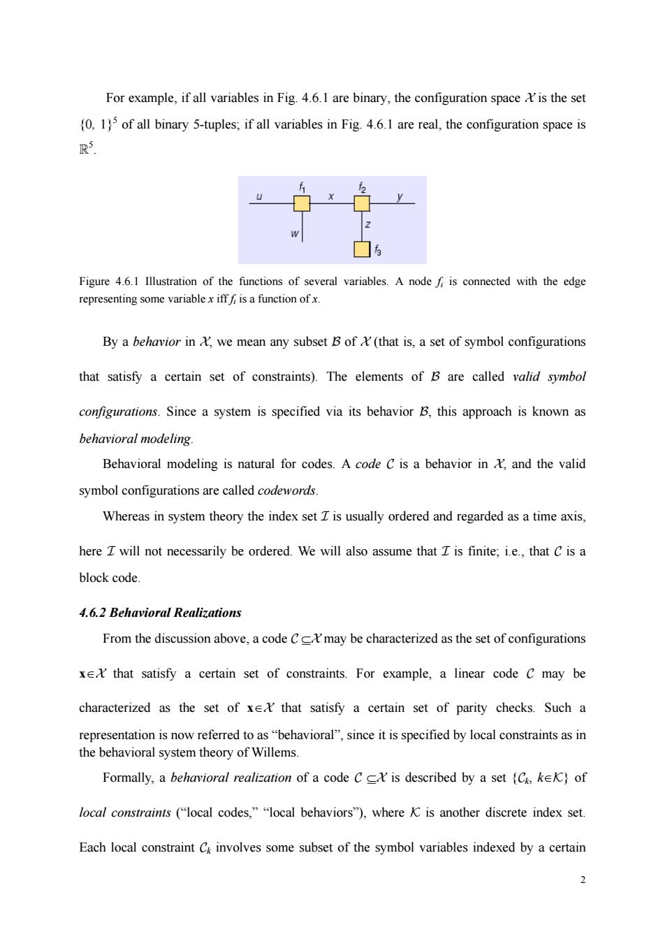
2 For example, if all variables in Fig. 4.6.1 are binary, the configuration space X is the set {0, 1}5 of all binary 5-tuples; if all variables in Fig. 4.6.1 are real, the configuration space is R5 . Figure 4.6.1 Illustration of the functions of several variables. A node fi is connected with the edge representing some variable x iff fi is a function of x. By a behavior in X, we mean any subset B of X (that is, a set of symbol configurations that satisfy a certain set of constraints). The elements of B are called valid symbol configurations. Since a system is specified via its behavior B, this approach is known as behavioral modeling. Behavioral modeling is natural for codes. A code C is a behavior in X, and the valid symbol configurations are called codewords. Whereas in system theory the index set I is usually ordered and regarded as a time axis, here I will not necessarily be ordered. We will also assume that I is finite; i.e., that C is a block code. 4.6.2 Behavioral Realizations From the discussion above, a code C ⊆X may be characterized as the set of configurations x∈X that satisfy a certain set of constraints. For example, a linear code C may be characterized as the set of x∈X that satisfy a certain set of parity checks. Such a representation is now referred to as “behavioral”, since it is specified by local constraints as in the behavioral system theory of Willems. Formally, a behavioral realization of a code C ⊆X is described by a set {Ck, k∈K} of local constraints (“local codes,” “local behaviors”), where K is another discrete index set. Each local constraint Ck involves some subset of the symbol variables indexed by a certain
subset (k),and defines a subset Gck)=Π光 of the corresponding local Cartesian product set).The local constraint thus defines a set of valid local configurations ("local codewords")xiI(k)C,where the notation xdenotes the projection of a configuration x onto the symbol variables indexed by(k) The code Cis then the set of all configurations that satisfy all local constraints C=xexx)C for all kek) For example,a linear code Cmay be characterized as the set of xe&that satisfy the parity-check equations <x,h>=0 for a certain set of check configurations (h.k).The symbol variables X,that are involved in the kth check are those for which h0.Each local code C is then a linear (m.n-1,2)single-parity-check (SPC)code, whose length nis equal to the number of symbols involved in C A behavioral realization has a nature graphical model,which in coding theory is called a Tanner graph. 4.6.3 Tanner Graph The above elementary linear behavioral realizations can be represented conveniently by a graphica Graph Notation A graph G is a triple consisting of a vertex set V(G),an edge set E(G),and a relation that associate with each edge two vertices called its endpoints. If vertex veV is an endpoint of edge eE,then v and e are incident.The degree of a vertex veVis the number of incident edges and will be denoted by d(v). A graph G is called regular when all of its vertices have degree r,i.e., v∈':d(v)=r Bipartite Graph:A bipartite graph is a graph whose vertices may be partitioned into two sets,and where edges may only connect two vertices not residing in the same set Amore precise definition is given below. 定义:若图G的节点集P可以划分为两个子集Y和'2:VU乃=',∩=p,使得 3
3 subset I(k), and defines a subset ( ) ( ) k i i k k ∈ ⊆ = ∏ I CX X of the corresponding local Cartesian product set X(k).The local constraint thus defines a set of valid local configurations (“local codewords”) x|() I ki k = {xi k , () ∈ ∈ I C } , where the notation x|I(k) denotes the projection of a configuration x onto the symbol variables Xi indexed by I(k). The code C is then the set of all configurations that satisfy all local constraints CX C K =∈ ∈ ∈ {x x| for all | () I k k k } For example, a linear code C ⊆X may be characterized as the set of x∈X that satisfy the parity-check equations , 0 < >= k x h for a certain set of check configurations { , } k h ∈ ∈ X K k . The symbol variables Xi that are involved in the kth check are those for which hki ≠0. Each local code Ck is then a linear (nk, nk-1, 2) single-parity-check (SPC) code, whose length nk is equal to the number of symbols involved in Ck. A behavioral realization has a nature graphical model, which in coding theory is called a Tanner graph. 4.6.3 Tanner Graph The above elementary linear behavioral realizations can be represented conveniently by a graphical model called Tanner graph. Graph Notation A graph G is a triple consisting of a vertex set V(G), an edge set E(G), and a relation Φ that associate with each edge two vertices called its endpoints. If vertex v∈V is an endpoint of edge e∈E, then v and e are incident. The degree of a vertex v∈V is the number of incident edges and will be denoted by d(v) . A graph G is called regular when all of its vertices have degree r; i.e., ∀∈ = v V dv r : ( ) . Bipartite Graph: A bipartite graph is a graph whose vertices may be partitioned into two sets, and where edges may only connect two vertices not residing in the same set. A more precise definition is given below. 定义: 若图 G 的节点集V 可以划分为两个子集V1和V2 : 12 12 V V VV V ∪= ∩= , φ ,使得
eeE,e的一个端,点属于K,另一个端点属于乃,则称G为二部图(bipartite graph). 若节点集匕中所有节点的度数都相同并且节点集,中所有节点的度数也都相同,则称G 为正则二部图(regular bipartite graph),否则称为非正则二部图(irregular bipartite graph), A cycle is a subgraph C=(VE)ofG=(V,E),whose vertices can be placed around a circle.The length ofa cycle Cis defined as /(C)E The girth of is the length of its shortest:g(G)C)where Cis the collection of all the cycles of G. A Tanmer graph is a bipartite graph in which a first set of vertices represents the symbol variables i,a second set of vertices represents the local constraints (C,ke),and an edge connects a variable vertex to a constraint vertex if and only if (iff)the corresponding symbol variable is volved in the ding local c aint.Fig.4.6.2 shows a Tanne graph for the (84,4)RMcode defined by the parity-check matrix 11110000 (4.1) 00001111 X0● 1●人 H ●大 为●< 狂 4● 5● H 6●Y 为● Fig.4.6.2 Tanner graph of parity-check representation for(8,4,4)code Here,symbol variables are represented by filled circles,and constraints (checks)by squares labeled by a+'sign.The four check nodes (vertices)represent the binary linear equations that each codeword must satisfy.In a valid codeword,the neighbors of every check
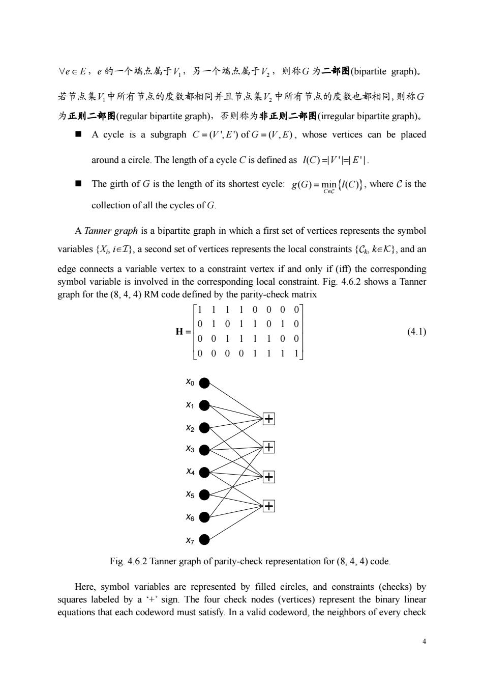
4 ∀e∈ E ,e 的一个端点属于V1,另一个端点属于V2 ,则称G 为二部图(bipartite graph)。 若节点集V1中所有节点的度数都相同并且节点集V2 中所有节点的度数也都相同,则称G 为正则二部图(regular bipartite graph),否则称为非正则二部图(irregular bipartite graph)。 A cycle is a subgraph ( ', ') of ( , ) C V E G VE = = , whose vertices can be placed around a circle. The length of a cycle C is defined as ( ) | ' | | ' | lC V E = = . The girth of G is the length of its shortest cycle: ( ) min ( ) { } C gG lC ∈ = C , where C is the collection of all the cycles of G. A Tanner graph is a bipartite graph in which a first set of vertices represents the symbol variables {Xi, i∈I}, a second set of vertices represents the local constraints {Ck, k∈K}, and an edge connects a variable vertex to a constraint vertex if and only if (iff) the corresponding symbol variable is involved in the corresponding local constraint. Fig. 4.6.2 shows a Tanner graph for the (8, 4, 4) RM code defined by the parity-check matrix 11110000 01011010 00111100 00001111 ⎡ ⎤ ⎢ ⎥ = ⎣ ⎦ H (4.1) x0 x1 x2 x3 x4 x5 x6 x7 Fig. 4.6.2 Tanner graph of parity-check representation for (8, 4, 4) code. Here, symbol variables are represented by filled circles, and constraints (checks) by squares labeled by a ‘+’ sign. The four check nodes (vertices) represent the binary linear equations that each codeword must satisfy. In a valid codeword, the neighbors of every check
node (i.e.the variables connected to the check by a single edge)must form a configuration with a binary sum of zero.Notice that this Tanner graph contains circles. The degree of a vertex is defined as the number of edges incident on it.Thus,the degree of a variable node is the number of local constraints(ie.,checks)that it is involved in,and the degree ofa constraint node is the number of variables that it involves.Clearly,in a Tanner grap the sum of the variable degrees isquoth sum of the ornt degreessine both qual to the number of edges in the graph. The degree of a variable or constraint will be defined as the degree of the corresponding graph vertex. In Fig.4.6.2.the local constraints consist of the following 4 parity-check equations (linear homogeneous equations). 6+写+x2+x3=0 +为+x+x6=0 2+x+x+x=0 ++x+x=0 4.6.4 General Linear Behavioral Realizations f Linear Block Codes The above elementary realizations can be generalized by letting symbol variable to vector spaces of dimension m over F.or more particularly m-tuples over Fg.The elements of a general linear behavioral realization of a linear(n,k,d)block code overF are as follows. A set of symbol m-tuple (x,i),where I denotes the (clustered)symbol variable index set.We define nm A set of state variable u-tuple (,where Jdenotes the state index set We defines=∑H, A set of (locally)linear constraint codes (C,kek)over F where K denotes the constraint index set,and each code C involves a certain subset of the symbol and state variables,indexed by (k)and )respectively. The symbol space is the Cartesian producthere the symbol alphabetsi.The state configuration space is the Cartesian product where the state alphabets (state spaces)s=F.A local configuration is a set 5
5 node (i.e., the variables connected to the check by a single edge) must form a configuration with a binary sum of zero. Notice that this Tanner graph contains circles. The degree of a vertex is defined as the number of edges incident on it. Thus, the degree of a variable node is the number of local constraints (i.e., checks) that it is involved in, and the degree of a constraint node is the number of variables that it involves. Clearly, in a Tanner graph the sum of the variable degrees is equal to the sum of the constraint degrees since both are equal to the number of edges in the graph. The degree of a variable or constraint will be defined as the degree of the corresponding graph vertex. In Fig. 4.6.2, the local constraints consist of the following 4 parity-check equations (linear homogeneous equations). 0123 1346 2345 4567 0 0 0 0 xxxx xxxx xxxx xxxx + ++= + ++= + ++= + ++= 4.6.4 General Linear Behavioral Realizations of Linear Block Codes [1][5] The above elementary realizations can be generalized by letting symbol variable to vector spaces of dimension m over Fq, or more particularly m-tuples over Fq. The elements of a general linear behavioral realization of a linear (n, k, d) block code over Fq are as follows. A set of symbol mi-tuple { ,} mi i q x i ∈ ∈ F I , where I denotes the (clustered) symbol variable index set. We define i i n m ∈ = ∑ I . A set of state variable μj-tuple { , } j j q s j μ ∈ ∈ F J , where J denotes the state index set. We define j j s μ ∈ = ∑ J . A set of (locally) linear constraint codes {Ck, k∈K} over Fq, where K denotes the constraint index set, and each code Ck involves a certain subset of the symbol and state variables, indexed by I(k) and J(k), respectively. The symbol configuration space is the Cartesian product i i∈ =∏ I X X , where the symbol alphabets , mi i q X I = ∈ F i . The state configuration space is the Cartesian product j j∈ =∏ J S S , where the state alphabets (state spaces) , j j q j μ S J = F ∈ . A local configuration is a set