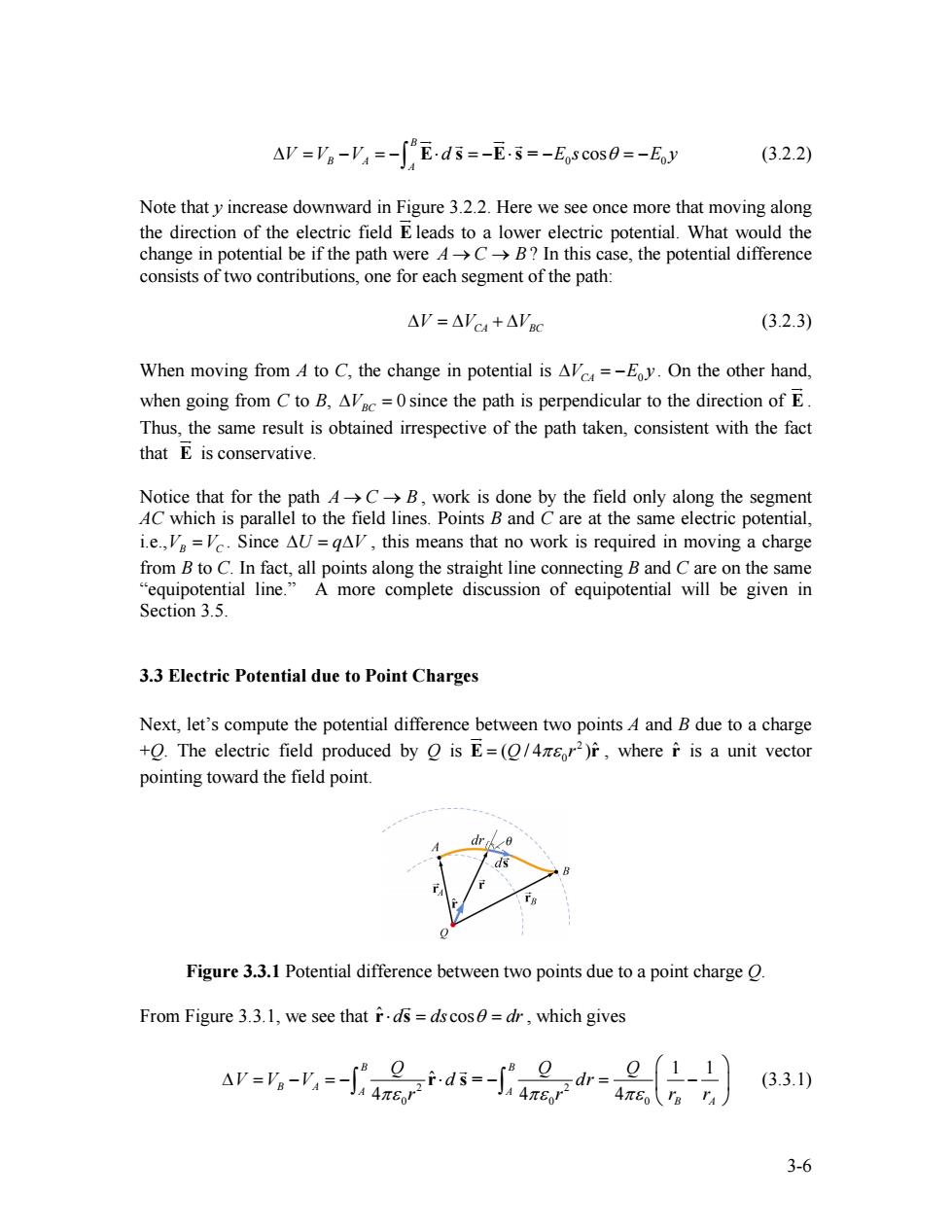
AV=V。-V4=-∫Eds=-Es=-E.scos0=-Ey (3.2.2) Note that y increase downward in Figure 3.2.2.Here we see once more that moving along the direction of the electric field E leads to a lower electric potential.What would the change in potential be if the path were A->C>B?In this case,the potential difference consists of two contributions,one for each segment of the path: AV=△'c4+A'C (3.2.3) When moving from A to C,the change in potential is Alc=-Eoy.On the other hand, when going from Cto B.AVc=0since the path is perpendicular to the direction of E. Thus,the same result is obtained irrespective of the path taken,consistent with the fact that E is conservative. Notice that for the path 4->C->B,work is done by the field only along the segment AC which is parallel to the field lines.Points B and C are at the same electric potential, i.e.,V=Vc.Since AU=gAv,this means that no work is required in moving a charge from B to C.In fact,all points along the straight line connecting B and C are on the same "equipotential line."A more complete discussion of equipotential will be given in Section 3.5. 3.3 Electric Potential due to Point Charges Next,let's compute the potential difference between two points A and B due to a charge +The electric field produced by o is E=(Q/4zr2)r,where i is a unit vector pointing toward the field point. dr, Figure 3.3.1 Potential difference between two points due to a point charge O. From Figure 3.3.1,we see that r.ds ds cos=dr,which gives ar=--r8d-2r-品-司 (3.3.1) 3-6
0 cos B B A A ∆V V=−= V − ⋅ d = − ⋅ −E s θ = −E y ∫ E s E s = 0 JG JG G G (3.2.2) Note that y increase downward in F gure 3.2.2. Here we see once more that moving along the direction of the electric field E i JG leads to a lower electric potential. What would the change in potential be if the path were ? In this case, the potential difference consists of two contributions, one for each segment of the path: A C → → B ∆V V = ∆ CA + ∆VBC (3.2.3) When moving from A to C, the change in potential is VCA E0 ∆ = − y . On the other hand, when going from C to B, ∆VBC = 0 since the path is perpendicular to the direction of E JG . Thus, the same result is obtained irrespective of the path taken, consistent with the fact that E JG is conservative. Notice that for the path , work is done by the field only along the segment AC which is parallel to the field lines. Points B and C are at the same electric potential, i.e., . Since , this means that no work is required in moving a charge from B to C. In fact, all points along the straight line connecting B and C are on the same “equipotential line.” A more complete discussion of equipotential will be given in Section 3.5. A C → → B VB =VC r ∆ = U q∆V 3.3 Electric Potential due to Point Charges Next, let’s compute the potential difference between two points A and B due to a charge +Q. The electric field produced by Q is 2 0 E = ( / Q 4πε r )ˆ JG , where is a unit vector pointing toward the field point. rˆ Figure 3.3.1 Potential difference between two points due to a point charge Q. From Figure 3.3.1, we see that r s ˆ ⋅ d d = s cosθ = dr G , which gives 2 2 0 0 0 1 1 ˆ 4 4 4 B B B A A A B A Q Q Q V V V d dr πε r r πε πε ⎛ ⎞ ∆ = − = − ⋅ − = ⎜ − ⎝ ⎠ ∫ ∫ r s =G r r ⎟ (3.3.1) 3-6
Once again,the potential differenceAl depends only on the endpoints,independent of the choice of path taken. As in the case of gravity,only the difference in electrical potential is physically meaningful,and one may choose a reference point and set the potential there to be zero. In practice,it is often convenient to choose the reference point to be at infinity,so that the electric potential at a point P becomes V=-fE.ds (3.3.2) With this reference,the electric potential at a distance r away from a point charge becomes V(r)= (3.3.3) 4π80r When more than one point charge is present,by applying the superposition principle,the total electric potential is simply the sum of potentials due to individual charges: m号-号 (3.3.4) A summary of comparison between gravitation and electrostatics is tabulated below: Gravitation Electrostatics Mass m Charge q Gravitational for Coulomb force F Gravitational field=F/m Electric field E=F/ Potential energy changeFd Potential energy changeF Gravitational potential Electrie Potential VEd For a source M:VGM Fora soue Q: IAU I=mgd (constant g) |△Ul=gEd(constant E) 3-7
Once again, the potential difference∆V depends only on the endpoints, independent of the choice of path taken. As in the case of gravity, only the difference in electrical potential is physically meaningful, and one may choose a reference point and set the potential there to be zero. In practice, it is often convenient to choose the reference point to be at infinity, so that the electric potential at a point P becomes P VP ∞ = − ⋅ d ∫ E s JG G (3.3.2) With this reference, the electric potential at a distance r away from a point charge Q becomes 0 1 ( ) 4 Q V r πε r = (3.3.3) When more than one point charge is present, by applying the superposition principle, the total electric potential is simply the sum of potentials due to individual charges: 0 1 ( ) 4 i i e i i i i q q V r k πε r r = = ∑ ∑ (3.3.4) A summary of comparison between gravitation and electrostatics is tabulated below: Gravitation Electrostatics Mass m Charge q Gravitational force 2 ˆ g Mm G r F r = − G Coulomb force 2 ˆ e e Qq k r F r = G Gravitational field / g F = g m G G Electric field / e E F = q G G Potential energy change B g A ∆ = U − ⋅ ∫ F s d G G Potential energy change B e A ∆ = U d − ⋅ ∫ F s G G Gravitational potential B g A V d = − ⋅ ∫ g s G G Electric Potential B A V d = − ⋅ ∫ E s G G For a source M: g GM V r = − For a source Q: e Q V k r = | | ∆ = Ug mgd (constant g G ) | | ∆U q = Ed (constant E ) JG 3-7

3.3.1 Potential Energy in a System of Charges If a system of charges is assembled by an external agent,thenAU=-W=+W.That is, the change in potential energy of the system is the work that must be put in by an external agent to assemble the configuration.A simple example is lifting a mass m through a height h.The work done by an external agent you,is +mgh (The gravitational field does work -mgh).The charges are brought in from infinity without acceleration i.e.they are at rest at the end of the process.Let's start with just two charges g and g2.Let the potential due to g at a point P be V(Figure 3.3.2). 92 12, 9○ Figure 3.3.2 Two point charges separated by a distance r2. The work W,done by an agent in bringing the second charge g2 from infinity to P is then W2=g2.(No work is required to set up the first charge and W=0).Since =g/4z2,where ri2 is the distance measured from g to p,we have 19192 U2=W=4π (3.3.5) If g and g2 have the same sign,positive work must be done to overcome the electrostatic repulsion and the potential energy of the system is positive,U20.On the other hand,if the signs are opposite,then U2 due to the attractive force between the charges. P 23 '12 93 91 13 Figure 3.3.3 A system of three point charges. To add a third charge g3 to the system(Figure 3.3.3),the work required is 3-8
3.3.1 Potential Energy in a System of Charges If a system of charges is assembled by an external agent, then∆U W = − = +Wext . That is, the change in potential energy of the system is the work that must be put in by an external agent to assemble the configuration. A simple example is lifting a mass m through a height h. The work done by an external agent you, is +mgh (The gravitational field does work ). The charges are brought in from infinity without acceleration i.e. they are at rest at the end of the process. Let’s start with just two charges and . Let the potential due to at a point be (Figure 3.3.2). −mgh 1 q 2 q 1 q P V1 Figure 3.3.2 Two point charges separated by a distance . 12 r The work done by an agent in bringing the second charge from infinity to P is then . (No work is required to set up the first charge and ). Since W2 2 q W q 2 = 2 V1 1 W = 0 1 1 0 12 V q = / 4πε r , where is the distance measured from to P, we have 12 r 1 q 1 2 12 2 0 12 1 4 q q U W πε r = = (3.3.5) If and q 1 q 2 have the same sign, positive work must be done to overcome the electrostatic repulsion and the potential energy of the system is positive, . On the other hand, if the signs are opposite, then due to the attractive force between the charges. 12 U > 0 12 U < 0 Figure 3.3.3 A system of three point charges. To add a third charge q3 to the system (Figure 3.3.3), the work required is 3-8
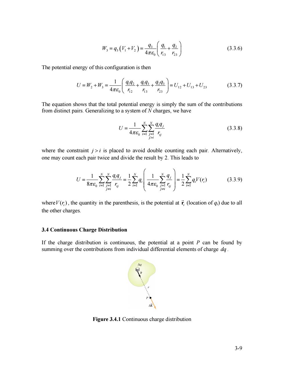
4+2 W=9+)=46a (3.3.6) The potential energy of this configuration is then U=W2+W3=- 1 9192+949+9294s =U2+U13+U23 (3.3.7 π8o12 1323 The equation shows that the total potential energy is simply the sum of the contributions from distinct pairs.Generalizing to a system of N charges,we have U=15949 (3.3.8) 4π台点 j> where the constraint j>i is placed to avoid double counting each pair.Alternatively, one may count each pair twice and divide the result by 2.This leads to 2 qV(r) (3.3.9) 8π台点有 whereV(),the quantity in the parenthesis,is the potential at r (location of gi)due to all the other charges. 3.4 Continuous Charge Distribution If the charge distribution is continuous,the potential at a point P can be found by summing over the contributions from individual differential elements of charge dq. E Figure 3.4.1 Continuous charge distribution 3-9
( ) 3 1 2 3 3 1 2 0 13 23 4 q q q W q V V πε r r ⎛ ⎞ = + = ⎜ + ⎝ ⎠⎟ (3.3.6) The potential energy of this configuration is then 1 2 1 3 2 3 2 3 12 13 23 0 12 13 23 1 4 q q q q q q U W W U U U πε rrr ⎛ ⎞ = + = ⎜ + + ⎟ = + + ⎝ ⎠ (3.3.7) The equation shows that the total potential energy is simply the sum of the contributions from distinct pairs. Generalizing to a system of N charges, we have 0 1 1 1 4 N N i j i j ij j i q q U πε = = r > = ∑∑ (3.3.8) where the constraint j > i is placed to avoid double counting each pair. Alternatively, one may count each pair twice and divide the result by 2. This leads to 0 0 1 1 1 1 1 1 1 1 1 ( ) 8 2 4 2 N N N N N i j j i i j ij i j ij i j i j i q q q U q πε = = r r = πε = = ≠ ≠ ⎛ ⎞ ⎜ ⎟ = = = ⎜ ⎟ ⎝ ⎠ ∑∑ ∑ ∑ ∑ i i qV r (3.3.9) where ( ) , the quantity in the parenthesis, is the potential at V ri i r G (location of qi) due to all the other charges. 3.4 Continuous Charge Distribution If the charge distribution is continuous, the potential at a point P can be found by summing over the contributions from individual differential elements of charge dq . Figure 3.4.1 Continuous charge distribution 3-9
Consider the charge distribution shown in Figure 3.4.1.Taking infinity as our reference point with zero potential,the electric potential at P due to dg is dv=-1 dq (3.4.1) 4π80r Summing over contributions from all differential elements,we have (3.4.2) 3.5 Deriving Electric Field from the Electric Potential In Eq.(3.1.9)we established the relation between E and V.If we consider two points which are separated by a small distance ds,the following differential form is obtained: dV=-E.ds (3.5.1) In Cartesian coordinates,E=Ei+Ej+E.k and ds=dxi+dyj+dzk,we have dV=(E.i+E,j+E.k)-(dxi+dyj+d=k)=E,dx+E,dy+E.d= (3.5.2) which implies av E ,E,= av Es (3.5.3) Ox Oy 0z By introducing a differential quantity called the"del(gradient)operator" i+jtok (3.5.4) the electric field can be written as ax E=-VV (3.5.5) Notice that V operates on a scalar quantity (electric potential)and results in a vector quantity (electric field).Mathematically,we can think of E as the negative of the gradient of the electric potential V.Physically,the negative sign implies that if 3-10
Consider the charge distribution shown in Figure 3.4.1. Taking infinity as our reference point with zero potential, the electric potential at P due to dq is 0 1 4 dq dV πε r = (3.4.1) Summing over contributions from all differential elements, we have 0 1 4 dq V πε r = ∫ (3.4.2) 3.5 Deriving Electric Field from the Electric Potential In Eq. (3.1.9) we established the relation between E JG and V. If we consider two points which are separated by a small distance ds G , the following differential form is obtained: dV = − ⋅ E d s JG G (3.5.1) In Cartesian coordinates, ˆ ˆ ˆ E i =++ E E x y Ez j k JG and ˆ ˆ ˆ d d s i = + x dyj+ dzk, G we have ( ) ( ) ˆ ˆ ˆ ˆ ˆ ˆ xyz x y z dV = + E i j E + E k ⋅ dxi + dyj+ dzk = E dx + E dy + E dz (3.5.2) which implies , , x y z V V E E E V x y z ∂ ∂ = − = − = − ∂ ∂ ∂ ∂ (3.5.3) By introducing a differential quantity called the “del (gradient) operator” ˆ ˆ ˆ x y z ∂ ∂ ∂ ∇ ≡ + ∂ ∂ ∂ i j+ k (3.5.4) the electric field can be written as ˆ ˆ ˆ ˆ ˆ ˆ ˆ ˆ ˆ xyz V V V E E E V V x y z x y z ⎛ ⎞ ∂ ∂ ∂ ⎛ ∂ ∂ ∂ ⎞ =++ = −⎜ ⎟ + = −⎜ + ⎟ = −∇ ⎝ ⎠ ∂ ∂ ∂ ⎝ ∂ ∂ ∂ ⎠ E i j k i + j k i + j k JG E = −∇V JG (3.5.5) Notice that ∇ operates on a scalar quantity (electric potential) and results in a vector quantity (electric field). Mathematically, we can think of E JG as the negative of the gradient of the electric potential V . Physically, the negative sign implies that if 3-10