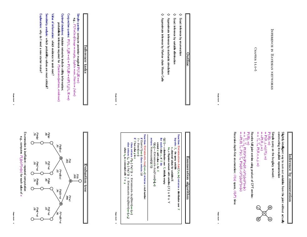
Explanation:why do I need a new starter motor? Sensitivity analysis:which probability values are most critical? Conjunctive queries:P(X:XE=e)=P(XE=e)P(XX E=e) Inference tasks *#*9829月38 Outline CHAPTER 14.4-5 INFERENCE IN BAYESIAN NETWORK Q Evaluation tree Enumeration algorithm Recursive depth-first enumeration:O(n)space,O()time Simple query on the burglary network: Inference by enumeration
Inference in Bayesian networks Chapter 14.4–5 Chapter 14.4–5 1 Outline ♦ Exact inference by enumeration ♦ Exact inference by variable elimination ♦ Approximate inference by stochastic simulation ♦ Approximate inference by Markov chain Monte Carlo Chapter 14.4–5 2 Inference tasks Simple queries: compute posterior marginal P(Xi |E = e) e.g., P(NoGas|Gauge = empty, Lights = on, Starts = false) Conjunctive queries: P(Xi , Xj |E = e) = P(Xi |E = e)P(Xj |Xi , E = e) Optimal decisions: decision networks include utility information; probabilistic inference required for P(outcome|action, evidence) Value of information: which evidence to seek next? Sensitivity analysis: which probability values are most critical? Explanation: why do I need a new starter motor? Chapter 14.4–5 3 Inference by enumeration Slightly intelligent way to sum out variables from the joint without actually constructing its explicit representation Simple query on the burglary network: B E J A M P(B|j, m) = P(B, j, m)/P(j, m) = αP(B, j, m) = α Σe Σa P(B, e, a, j, m) Rewrite full joint entries using product of CPT entries: P(B|j, m) = α Σe Σa P(B)P(e)P(a|B, e)P(j|a)P(m|a) = αP(B) Σe P(e) Σa P(a|B, e)P(j|a)P(m|a) Recursive depth-first enumeration: O(n) space, O(d n ) time Chapter 14.4–5 4 Enumeration algorithm function Enumeration-Ask(X, e, bn) returns a distribution over X inputs: X, the query variable e, observed values for variables E bn, a Bayesian network with variables {X} ∪ E ∪ Y Q(X ) ← a distribution over X, initially empty for each value xi of X do extend e with value xi for X Q(xi) ← Enumerate-All(Vars[bn], e) return Normalize(Q(X )) function Enumerate-All(vars, e) returns a real number if Empty?(vars) then return 1.0 Y ← First(vars) if Y has value y in e then return P(y | Pa(Y )) × Enumerate-All(Rest(vars), e) else return P y P(y | Pa(Y )) × Enumerate-All(Rest(vars), ey ) where ey is e extended with Y = y Chapter 14.4–5 5 Evaluation tree .70 P(m|a) .90 P(j|a) .01 P(m| a) .05 P(j| a) .70 P(m|a) .90 P(j|a) .01 P(m| a) .05 P(j| a) .001 P(b) .002 P(e) .998 P( e) .95 P(a|b,e) .06 P( a|b, e) .05 P( a|b,e) .94 P(a|b, e) Enumeration is inefficient: repeated computation e.g., computes P(j|a)P(m|a) for each value of e Chapter 14.4–5 6
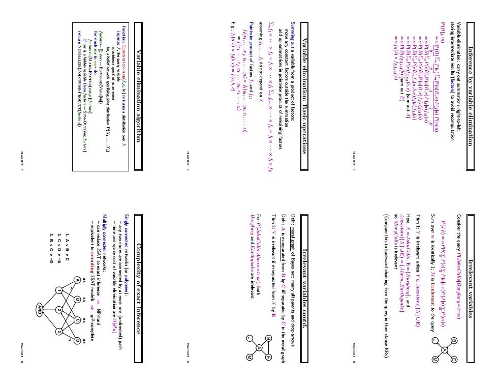
ssuming do not depend on P(Bl3.m) Variable elimination algorithm mingout a variable from a product of factors: Variable elimination:Basic operations Inference by variable elimination 1.A vB v C equivalent to counting 3SAT model#P-complete can reduce 3SAT to exact inference NP.hard Complexity of exact inference Thm 2:Y is irrelevant if m-separated from X by E Defn:A from B by Ciff separated by Cin the moral grap Irrelevant variables contd. (Compare this to backward chaining from the query in Hom dlause KBs) Sum over m is ickentically 1:is irrelevant to the query Consider the query P(JohnCalls Bur glary=true) Irrelevant variables Q
Inference by variable elimination Variable elimination: carry out summations right-to-left, storing intermediate results (factors) to avoid recomputation P(B|j, m) = α P(B) | {z } B Σe P(e) | {z } E Σa P(a|B, e) | {z } A P(j|a) | {z } J P(m|a) | {z } M = αP(B)ΣeP(e)ΣaP(a|B, e)P(j|a)fM(a) = αP(B)ΣeP(e)ΣaP(a|B, e)fJ(a)fM(a) = αP(B)ΣeP(e)ΣafA(a, b, e)fJ(a)fM(a) = αP(B)ΣeP(e)fA¯JM(b, e) (sum out A) = αP(B)fE¯AJ¯ M(b) (sum out E) = αfB(b) × fE¯AJ¯ M(b) Chapter 14.4–5 7 Variable elimination: Basic operations Summing out a variable from a product of factors: move any constant factors outside the summation add up submatrices in pointwise product of remaining factors Σxf1 × · · · × fk = f1 × · · · × fi Σx fi+1 × · · · × fk = f1 × · · · × fi × fX¯ assuming f1, . . . , fi do not depend on X Pointwise product of factors f1 and f2: f1(x1, . . . , xj , y1, . . . , yk) × f2(y1, . . . , yk, z1, . . . , zl) = f(x1, . . . , xj , y1, . . . , yk, z1, . . . , zl) E.g., f1(a, b) × f2(b, c) = f(a, b, c) Chapter 14.4–5 8 Variable elimination algorithm function Elimination-Ask(X, e, bn) returns a distribution over X inputs: X, the query variable e, evidence specified as an event bn, a belief network specifying joint distribution P(X1, . . . , Xn) factors ← [ ]; vars ← Reverse(Vars[bn]) for each var in vars do factors ← [Make-Factor(var , e)|factors] if var is a hidden variable then factors ← Sum-Out(var,factors) return Normalize(Pointwise-Product(factors)) Chapter 14.4–5 9 Irrelevant variables Consider the query P(JohnCalls|Burglary = true) B E J A M P(J|b) = αP(b) e X P(e) a X P(a|b, e)P(J|a) m X P(m|a) Sum over m is identically 1; M is irrelevant to the query Thm 1: Y is irrelevant unless Y ∈ Ancestors({X}∪ E) Here, X = JohnCalls, E = {Burglary}, and Ancestors({X}∪ E) = {Alarm, Earthquake} so MaryCalls is irrelevant (Compare this to backward chaining from the query in Horn clause KBs) Chapter 14.4–5 10 Irrelevant variables contd. Defn: moral graph of Bayes net: marry all parents and drop arrows Defn: A is m-separated from B by C iff separated by C in the moral graph Thm 2: Y is irrelevant if m-separated from X by E B E J A M For P(JohnCalls|Alarm = true), both Burglary and Earthquake are irrelevant Chapter 14.4–5 11 Complexity of exact inference Singly connected networks (or polytrees): – any two nodes are connected by at most one (undirected) path – time and space cost of variable elimination are O(d kn) Multiply connected networks: – can reduce 3SAT to exact inference ⇒ NP-hard – equivalent to counting 3SAT models ⇒ #P-complete A B C D 1 2 3 AND 0.5 0.5 0.5 0.5 L L L L 3. B v C v D 2. C v D v A 1. A v B v C Chapter 14.4–5 12
Basic idea 酮 Sampling from an empty network whose stationary dist ribution is the true posterior -Mark chain Monte Cark(MCMC):samplefrom a stochastic proces Inference by stochastic simulation 图E S R P(WIS.R) Example P(WIS.R Example 可
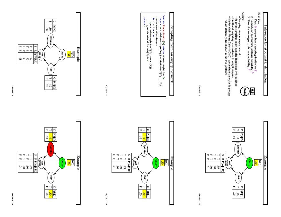
Inference by stochastic simulation Basic idea: 1) Draw N samples from a sampling distribution S Coin 0.5 2) Compute an approximate posterior probability Pˆ 3) Show this converges to the true probability P Outline: – Sampling from an empty network – Rejection sampling: reject samples disagreeing with evidence – Likelihood weighting: use evidence to weight samples – Markov chain Monte Carlo (MCMC): sample from a stochastic process whose stationary distribution is the true posterior Chapter 14.4–5 13 Sampling from an empty network function Prior-Sample(bn) returns an event sampled from bn inputs: bn, a belief network specifying joint distribution P(X1, . . . , Xn) x ← an event with n elements for i = 1 to n do xi ← a random sample from P(Xi | parents(Xi)) given the values of Parents(Xi) in x return x Chapter 14.4–5 14 Example Cloudy Rain Sprinkler Grass Wet F T C .20 .80 P(R|C) F T C .50 .10 P(S|C) S R T T T F F T F F .90 .90 .99 P(W|S,R) P(C) .50 .01 Chapter 14.4–5 15 Example Cloudy Rain Sprinkler Grass Wet F T C .20 .80 P(R|C) F T C .50 .10 P(S|C) S R T T T F F T F F .90 .90 .99 P(W|S,R) P(C) .50 .01 Chapter 14.4–5 16 Example Cloudy Rain Sprinkler Grass Wet F T C .20 .80 P(R|C) F T C .50 .10 P(S|C) S R T T T F F T F F .90 .90 .99 P(W|S,R) P(C) .50 .01 Chapter 14.4–5 17 Example Cloudy Rain Sprinkler Grass Wet F T C .20 .80 P(R|C) F T C .50 .10 P(S|C) S R T T T F F T F F .90 .90 .99 P(W|S,R) P(C) .50 .01 Chapter 14.4–5 18

c P(SC) c P(SC) 三88 S RPWIS,R) 色888 P(e)drops off exp Hence Then we have ples have Sp with numbe r of evidence Analysis of rejection sampling P(fain|Sprindfer=trwe)=NORMALIZE(()=(02%6.0.70) Rejection sampling Let Ns)be the number of samples generated for evn Sampling from an empty network contd
Example Cloudy Rain Sprinkler Grass Wet F T C .20 .80 P(R|C) F T C .50 .10 P(S|C) S R T T T F F T F F .90 .90 .99 P(W|S,R) P(C) .50 .01 Chapter 14.4–5 19 Example Cloudy Rain Sprinkler Grass Wet F T C .20 .80 P(R|C) F T C .50 .10 P(S|C) S R T T T F F T F F .90 .90 .99 P(W|S,R) P(C) .50 .01 Chapter 14.4–5 20 Example Cloudy Rain Sprinkler Grass Wet F T C .20 .80 P(R|C) F T C .50 .10 P(S|C) S R T T T F F T F F .90 .90 .99 P(W|S,R) P(C) .50 .01 Chapter 14.4–5 21 Sampling from an empty network contd. Probability that PriorSample generates a particular event SPS(x1 . . . xn) = Πi n = 1P(xi |parents(Xi)) = P(x1 . . . xn) i.e., the true prior probability E.g., SPS(t, f,t,t) = 0.5 × 0.9 × 0.8 × 0.9 = 0.324 = P(t, f,t,t) Let NPS(x1 . . . xn) be the number of samples generated for event x1, . . . , xn Then we have N→∞ lim Pˆ(x1, . . . , xn) = N→∞ lim NPS(x1, . . . , xn)/N = SPS(x1, . . . , xn) = P(x1 . . . xn) That is, estimates derived from PriorSample are consistent Shorthand: Pˆ(x1, . . . , xn) ≈ P(x1 . . . xn) Chapter 14.4–5 22 Rejection sampling Pˆ (X|e) estimated from samples agreeing with e function Rejection-Sampling(X, e, bn,N) returns an estimate of P(X |e) local variables: N, a vector of counts over X, initially zero for j = 1 to N do x ← Prior-Sample(bn) if x is consistent with e then N[x] ← N[x]+1 where x is the value of X in x return Normalize(N[X]) E.g., estimate P(Rain|Sprinkler = true) using 100 samples 27 samples have Sprinkler = true Of these, 8 have Rain = true and 19 have Rain = false. Pˆ (Rain|Sprinkler = true) = Normalize(h8, 19i) = h0.296, 0.704i Similar to a basic real-world empirical estimation procedure Chapter 14.4–5 23 Analysis of rejection sampling Pˆ (X|e) = αNPS(X, e) (algorithm defn.) = NPS(X, e)/NPS(e) (normalized by NPS(e)) ≈ P(X, e)/P(e) (property of PriorSample) = P(X|e) (defn. of conditional probability) Hence rejection sampling returns consistent posterior estimates Problem: hopelessly expensive if P(e) is small P(e) drops off exponentially with number of evidence variables! Chapter 14.4–5 24
S RRWISR) Likelihood weighting example Likelihood weighting example Likelihood weighting 888 Likelihood weighting example 可 Likelihood weighting example Likelihood weighting example
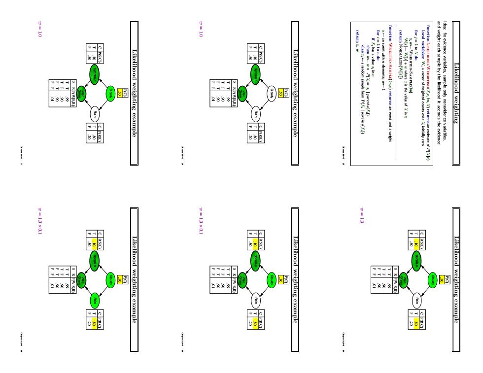
Likelihood weighting Idea: fix evidence variables, sample only nonevidence variables, and weight each sample by the likelihood it accords the evidence function Likelihood-Weighting(X, e, bn,N) returns an estimate of P(X |e) local variables: W, a vector of weighted counts over X, initially zero for j = 1 to N do x,w ←Weighted-Sample(bn) W[x ] ←W[x ] + w where x is the value of X in x return Normalize(W[X ]) function Weighted-Sample(bn, e) returns an event and a weight x ← an event with n elements; w ← 1 for i = 1 to n do if Xi has a value xi in e then w ← w × P(Xi = xi | parents(Xi)) else xi ← a random sample from P(Xi | parents(Xi)) return x, w Chapter 14.4–5 25 Likelihood weighting example Cloudy Rain Sprinkler Grass Wet F T C .20 .80 P(R|C) F T C .50 .10 P(S|C) S R T T T F F T F F .90 .90 .99 P(W|S,R) P(C) .50 .01 w = 1.0 Chapter 14.4–5 26 Likelihood weighting example Cloudy Rain Sprinkler Grass Wet F T C .20 .80 P(R|C) F T C .50 .10 P(S|C) S R T T T F F T F F .90 .90 .99 P(W|S,R) P(C) .50 .01 w = 1.0 Chapter 14.4–5 27 Likelihood weighting example Cloudy Rain Sprinkler Grass Wet F T C .20 .80 P(R|C) F T C .50 .10 P(S|C) S R T T T F F T F F .90 .90 .99 P(W|S,R) P(C) .50 .01 w = 1.0 Chapter 14.4–5 28 Likelihood weighting example Cloudy Rain Sprinkler Grass Wet F T C .20 .80 P(R|C) F T C .50 .10 P(S|C) S R T T T F F T F F .90 .90 .99 P(W|S,R) P(C) .50 .01 w = 1.0 × 0.1 Chapter 14.4–5 29 Likelihood weighting example Cloudy Rain Sprinkler Grass Wet F T C .20 .80 P(R|C) F T C .50 .10 P(S|C) S R T T T F F T F F .90 .90 .99 P(W|S,R) P(C) .50 .01 w = 1.0 × 0.1 Chapter 14.4–5 30