Dynamic Bayesian network Hidden Markov model Time and uncertainty Time and uncertainty Kalman filters (a brief mention Outlin CHAPTER 15,SECTIONS 1- TEMPORAL PROBABILITY MODE Fr-arder Inference tasks Sensor Markov assumption:P(EX E-1)-P(EX) asumption:X depends on bounded subset of X Markov processes (Markoy chains) rrF
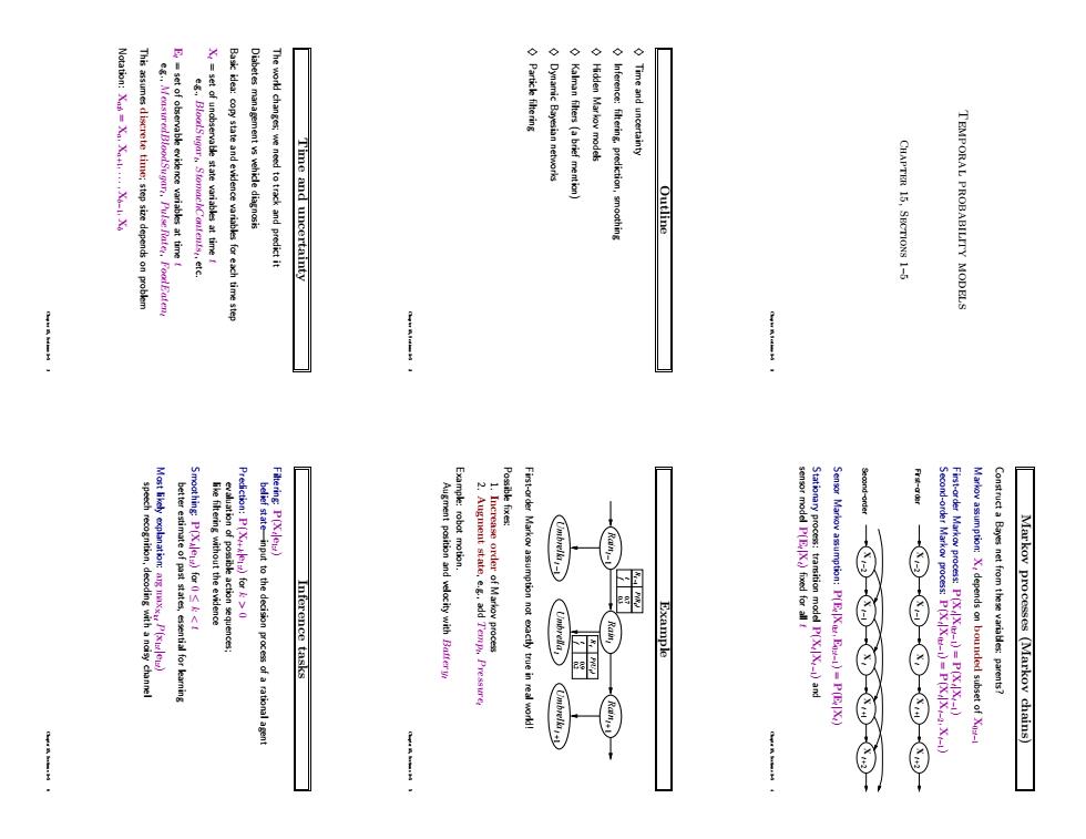
Temporal probability models Chapter 15, Sections 1–5 Chapter 15, Sections 1–5 1 Outline ♦ Time and uncertainty ♦ Inference: filtering, prediction, smoothing ♦ Hidden Markov models ♦ Kalman filters (a brief mention) ♦ Dynamic Bayesian networks ♦ Particle filtering Chapter 15, Sections 1–5 2 Time and uncertainty The world changes; we need to track and predict it Diabetes management vs vehicle diagnosis Basic idea: copy state and evidence variables for each time step Xt = set of unobservable state variables at time t e.g., BloodSugart , StomachContentst , etc. Et = set of observable evidence variables at time t e.g., MeasuredBloodSugart , PulseRatet , FoodEatent This assumes discrete time; step size depends on problem Notation: Xa:b = Xa, Xa+1, . . . , Xb−1, Xb Chapter 15, Sections 1–5 3 Markov processes (Markov chains) Construct a Bayes net from these variables: parents? Markov assumption: Xt depends on bounded subset of X0:t−1 First-order Markov process: P(Xt |X0:t−1) = P(Xt |Xt−1) Second-order Markov process: P(Xt |X0:t−1) = P(Xt |Xt−2, Xt−1) X t −1 X t X t −2 X t +1 X t +2 X t −1 X t X t −2 X t +1 X t +2 Senso Second−order First−order r Markov assumption: P(Et |X0:t , E0:t−1) = P(Et |Xt) Stationary process: transition model P(Xt |Xt−1) and sensor model P(Et |Xt) fixed for all t Chapter 15, Sections 1–5 4 Example t Rain t Umbrella Raint −1 Umbrellat −1 Raint +1 Umbrellat +1 Rt −1 t P(R ) 0.3 f 0.7 t t R t P(U ) 0.9 t 0.2 f First-order Markov assumption not exactly true in real world! Possible fixes: 1. Increase order of Markov process 2. Augment state, e.g., add Tempt , Pressuret Example: robot motion. Augment position and velocity with Batteryt Chapter 15, Sections 1–5 5 Inference tasks Filtering: P(Xt |e1:t) belief state—input to the decision process of a rational agent Prediction: P(Xt+k|e1:t) for k > 0 evaluation of possible action sequences; like filtering without the evidence Smoothing: P(Xk|e1:t) for 0 ≤ k < t better estimate of past states, essential for learning Most likely explanation: arg maxx1:t P(x1:t |e1:t) speech recognition, decoding with a noisy channel Chapter 15, Sections 1–5 6
P(Xxle)P(Xe P()P(+X) Divide evidence e intoe Smoothing T 5) Aim:devise a recursive state estimation algorithm Filtering iterbi examplo kenticaltoflteringexceptreplaced by Most likely explanation Smoothing example 的
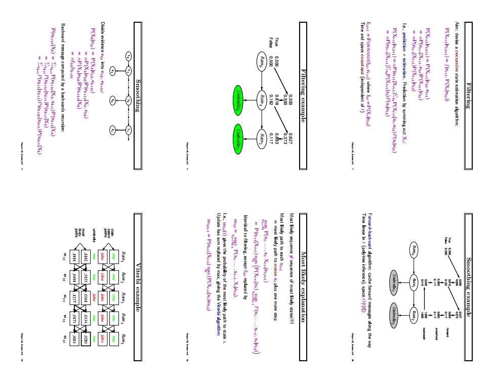
Filtering Aim: devise a recursive state estimation algorithm: P(Xt+1|e1:t+1) = f(et+1, P(Xt |e1:t)) P(Xt+1|e1:t+1) = P(Xt+1|e1:t , et+1) = αP(et+1|Xt+1, e1:t)P(Xt+1|e1:t) = αP(et+1|Xt+1)P(Xt+1|e1:t) I.e., prediction + estimation. Prediction by summing out Xt : P(Xt+1|e1:t+1) = αP(et+1|Xt+1)ΣxtP(Xt+1|xt , e1:t)P(xt |e1:t) = αP(et+1|Xt+1)ΣxtP(Xt+1|xt)P(xt |e1:t) f1:t+1 = Forward(f1:t , et+1) where f1:t = P(Xt |e1:t) Time and space constant (independent of t) Chapter 15, Sections 1–5 7 Filtering example Rain1 Umbrella1 Rain2 Umbrella2 Rain0 0.182 0.818 0.117 0.883 0.373 0.627 False True 0.500 0.500 0.500 0.500 Chapter 15, Sections 1–5 8 Smoothing X 0 X 1 1 E Ek t E t X X k Divide evidence e1:t into e1:k, ek+1:t : P(Xk|e1:t) = P(Xk|e1:k, ek+1:t) = αP(Xk|e1:k)P(ek+1:t |Xk, e1:k) = αP(Xk|e1:k)P(ek+1:t |Xk) = αf1:kbk+1:t Backward message computed by a backwards recursion: P(ek+1:t |Xk) = Σxk+1P(ek+1:t |Xk, xk+1)P(xk+1|Xk) = Σxk+1P(ek+1:t |xk+1)P(xk+1|Xk) = Σxk+1P(ek+1|xk+1)P(ek+2:t |xk+1)P(xk+1|Xk) Chapter 15, Sections 1–5 9 Smoothing example Rain1 Umbrella1 Rain2 Umbrella2 Rain0 False True 0.182 0.818 0.117 0.883 0.373 0.627 0.500 0.500 0.500 0.500 1.000 1.000 0.410 0.690 0.117 0.883 backward smoothed forward 0.117 0.883 Forward–backward algorithm: cache forward messages along the way Time linear in t (polytree inference), space O(t|f|) Chapter 15, Sections 1–5 10 Most likely explanation Most likely sequence 6= sequence of most likely states!!!! Most likely path to each xt+1 = most likely path to some xt plus one more step x max 1...xt P(x1, . . . , xt , Xt+1|e1:t+1) = P(et+1|Xt+1) max xt P(Xt+1|xt) max x1...xt−1 P(x1, . . . , xt−1, xt |e1:t) Identical to filtering, except f1:t replaced by m1:t = max x1...xt−1 P(x1, . . . , xt−1, Xt |e1:t), I.e., m1:t(i) gives the probability of the most likely path to state i. Update has sum replaced by max, giving the Viterbi algorithm: m1:t+1 = P(et+1|Xt+1) max xt (P(Xt+1|xt)m1:t) Chapter 15, Sections 1–5 11 Viterbi example Rain1 Rain2 Rain3 Rain4 Rain5 false true false true false true false true false true .8182 .5155 .0361 .0334 .0210 .1818 .0491 .1237 .0173 .0024 m 1:1 m 1:5 m 1:4 m 1:3 m 1:2 paths likely most umbrella paths space state true true true false true Chapter 15, Sections 1–5 12
82333 Country dance algorithm Country dance algorithm rd-backward arithm need time()and space ( Forward and backward mesa cdumn vectors diagonal elementsP Hidden Markoy models 0 会 ① Country dance algorithm Country dance algorithm Algorithm:rward pass computes pass does f b Country dance algorithm
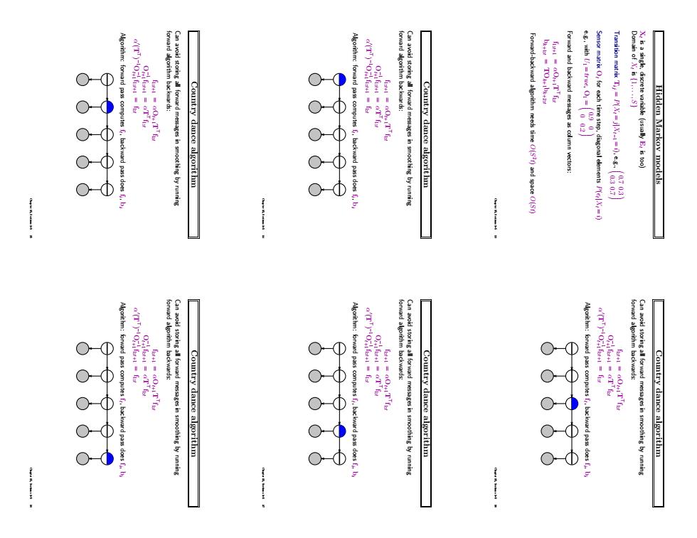
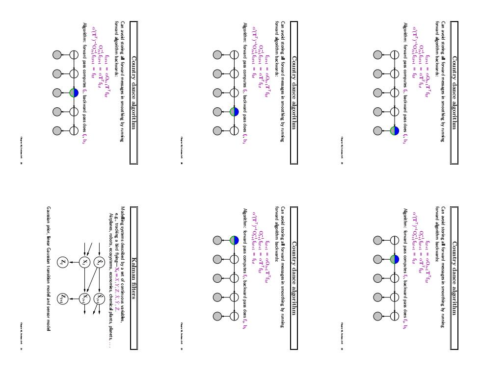
Hidden Markov models Xt is a single, discrete variable (usually Et is too) Domain of Xt is {1, . . . , S} Transition matrix Tij = P(Xt = j|Xt−1 = i), e.g., 0.7 0.3 0.3 0.7 Sensor matrix Ot for each time step, diagonal elements P(et |Xt = i) e.g., with U1 = true, O1 = 0.9 0 0 0.2 Forward and backward messages as column vectors: f1:t+1 = αOt+1T > f1:t bk+1:t = TOk+1bk+2:t Forward-backward algorithm needs time O(S 2 t) and space O(St) Chapter 15, Sections 1–5 13 Country dance algorithm Can avoid storing all forward messages in smoothing by running forward algorithm backwards: f1:t+1 = αOt+1T > f1:t O−1 t+1 f1:t+1 = αT > f1:t α 0 (T > ) − O1 −1 t+1 f1:t+1 = f1:t Algorithm: forward pass computes ft , backward pass does fi , bi Chapter 15, Sections 1–5 14 Country dance algorithm Can avoid storing all forward messages in smoothing by running forward algorithm backwards: f1:t+1 = αOt+1T > f1:t O−1 t+1 f1:t+1 = αT > f1:t α 0 (T > ) − O1 −1 t+1 f1:t+1 = f1:t Algorithm: forward pass computes ft , backward pass does fi , bi Chapter 15, Sections 1–5 15 Country dance algorithm Can avoid storing all forward messages in smoothing by running forward algorithm backwards: f1:t+1 = αOt+1T > f1:t O−1 t+1 f1:t+1 = αT > f1:t α 0 (T > ) − O1 −1 t+1 f1:t+1 = f1:t Algorithm: forward pass computes ft , backward pass does fi , bi Chapter 15, Sections 1–5 16 Country dance algorithm Can avoid storing all forward messages in smoothing by running forward algorithm backwards: f1:t+1 = αOt+1T > f1:t O−1 t+1 f1:t+1 = αT > f1:t α 0 (T > ) − O1 −1 t+1 f1:t+1 = f1:t Algorithm: forward pass computes ft , backward pass does fi , bi Chapter 15, Sections 1–5 17 Country dance algorithm Can avoid storing all forward messages in smoothing by running forward algorithm backwards: f1:t+1 = αOt+1T > f1:t O−1 t+1 f1:t+1 = αT > f1:t α 0 (T > ) − O1 −1 t+1 f1:t+1 = f1:t Algorithm: forward pass computes ft , backward pass does fi , bi Chapter 15, Sections 1–5 18
3533 0 ① Country dance algorithm Country dance algorithm Algorithm:forward pass computes,backward pass does b Country dance algorithm linear Gau (TT)O=fia model and sen Kalman filters m1 Country dance algorithm Country dance algorithm
Country dance algorithm Can avoid storing all forward messages in smoothing by running forward algorithm backwards: f1:t+1 = αOt+1T > f1:t O−1 t+1 f1:t+1 = αT > f1:t α 0 (T > ) − O1 −1 t+1 f1:t+1 = f1:t Algorithm: forward pass computes ft , backward pass does fi , bi Chapter 15, Sections 1–5 19 Country dance algorithm Can avoid storing all forward messages in smoothing by running forward algorithm backwards: f1:t+1 = αOt+1T > f1:t O−1 t+1 f1:t+1 = αT > f1:t α 0 (T > ) − O1 −1 t+1 f1:t+1 = f1:t Algorithm: forward pass computes ft , backward pass does fi , bi Chapter 15, Sections 1–5 20 Country dance algorithm Can avoid storing all forward messages in smoothing by running forward algorithm backwards: f1:t+1 = αOt+1T > f1:t O−1 t+1 f1:t+1 = αT > f1:t α 0 (T > ) − O1 −1 t+1 f1:t+1 = f1:t Algorithm: forward pass computes ft , backward pass does fi , bi Chapter 15, Sections 1–5 21 Country dance algorithm Can avoid storing all forward messages in smoothing by running forward algorithm backwards: f1:t+1 = αOt+1T > f1:t O−1 t+1 f1:t+1 = αT > f1:t α 0 (T > ) − O1 −1 t+1 f1:t+1 = f1:t Algorithm: forward pass computes ft , backward pass does fi , bi Chapter 15, Sections 1–5 22 Country dance algorithm Can avoid storing all forward messages in smoothing by running forward algorithm backwards: f1:t+1 = αOt+1T > f1:t O−1 t+1 f1:t+1 = αT > f1:t α 0 (T > ) − O1 −1 t+1 f1:t+1 = f1:t Algorithm: forward pass computes ft , backward pass does fi , bi Chapter 15, Sections 1–5 23 Kalman filters Modelling systems described by a set of continuous variables, e.g., tracking a bird flying—Xt = X, Y, Z, X˙ , Y˙ , Z˙ . Airplanes, robots, ecosystems, economies, chemical plants, planets, . . . t Z t+1 Z t X t+1 X t X t+1 X Gaussian prior, linear Gaussian transition model and sensor model Chapter 15, Sections 1–5 24
is Gaussian sequence,so compute offlin General Kalman update +8+元 Gaussian random walk ons.d.se Simple I-D example Here P(X)s multivariate Gaussian N for al t Prediction step:if P()is Gaussian,then RA113-25 Updating Gaussian distributions Where it breaks 2-D tracking example:smoothing 2-D tracking example:filtering
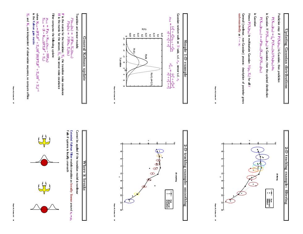
Updating Gaussian distributions Prediction step: if P(Xt |e1:t) is Gaussian, then prediction P(Xt+1|e1:t) = Z xt P(Xt+1|xt)P(xt |e1:t) dxt is Gaussian. If P(Xt+1|e1:t) is Gaussian, then the updated distribution P(Xt+1|e1:t+1) = αP(et+1|Xt+1)P(Xt+1|e1:t) is Gaussian Hence P(Xt |e1:t) is multivariate Gaussian N(µt , Σt) for all t General (nonlinear, non-Gaussian) process: description of posterior grows unboundedly as t → ∞ Chapter 15, Sections 1–5 25 Simple 1-D example Gaussian random walk on X–axis, s.d. σx, sensor s.d. σz µt+1 = (σt 2 + σx 2 )zt+1 + σz 2µt σt 2 + σx 2 + σz 2 σt+1 2 = (σt 2 + σx 2 )σz 2 σt 2 + σx 2 + σz 2 0 0.05 0.1 0.15 0.2 0.25 0.3 0.35 0.4 0.45 -8 -6 -4 -2 0 2 4 6 8 P(X) X position P(x0) P(x1) P(x1 | z1=2.5) z1 * Chapter 15, Sections 1–5 26 General Kalman update Transition and sensor models: P(xt+1|xt) = N(Fxt , Σx)(xt+1) P(zt |xt) = N(Hxt , Σz)(zt) F is the matrix for the transition; Σx the transition noise covariance H is the matrix for the sensors; Σz the sensor noise covariance Filter computes the following update: µt+1 = Fµt + Kt+1(zt+1 − HFµt ) Σt+1 = (I − Kt+1)(FΣtF > + Σx) where Kt+1 = (FΣtF > + Σx)H> (H(FΣtF > + Σx)H> + Σz) −1 is the Kalman gain matrix Σt and Kt are independent of observation sequence, so compute offline Chapter 15, Sections 1–5 27 2-D tracking example: filtering 8 10 12 14 16 18 20 22 24 26 6 7 8 9 10 11 12 X Y 2D filtering filtered observed true Chapter 15, Sections 1–5 28 2-D tracking example: smoothing 8 10 12 14 16 18 20 22 24 26 6 7 8 9 10 11 12 X Y 2D smoothing smoothed observed true Chapter 15, Sections 1–5 29 Where it breaks Cannot be applied if the transition model is nonlinear Extended Kalman Filter models transition as locally linear around xt = µt Fails if systems is locally unsmooth Chapter 15, Sections 1–5 30