RSC component encoder generated by an information sequence withwmin=2.Then we have the following definition of the effective free distance for (un-punctured)turbo codes. free.eff 2*2 The effective free distance plays a role similar to that of the free distance for convolutional codes. 4.2.4 Structure ofTurbo Decoder 如前所述,采用删余技术时tubo编码器在k时刻的输出为c=(c,cf),其中 c由c和cP交替组成。如果采用BPSK调制,则信道上的发送符号为 x=(x,x)=(2c-l)WE,(2c-1)WE,),1≤k≤N 经过信道传输、相干解调,接收机匹配滤波器在k时刻的输出采样值为y。=(Oy,y), 译码器的任务就是从此接收序列来估计发送符号。 Tubo码译码器的基本结构如图4.9所示。它由两个软输入软输出(SIS0)译码器 decl和dcc2串行级联组成,交织器与编码器中所使用的交织器相同。译码器dccl对分 量码R$C1进行最佳译码,产生关于信息序列Ⅱ中每一比特的后验概率信息,并将其中 的“新信息”经过交织送给dec2:译码器dec2将此信息作为先验信息,对分量码RSC2 进行最佳译码,产生关于交织后的信息序列中每一比特的后验概率信息,然后将其中的 “新信息”经过解交织送给decl,进行下一次译码。这样,经过多次迭代,decl或dec2 新产生的外信息趋于稳定,后验概率比渐进值逼近于对整个码的最大似然译码。 When the series of iterations halts,after either a fixed number of iterations or when a termination criterion is satisfied,the output from the turbo decoder is given by the de-interleaved a-posteriori LLRs of the second component decoder.The sign of these a-posteriori LLRs gives the hard decision output 帮交钢、以 w(L) w(y) y DECI 门决 交织 图4.9 Turbo码译码器的结构.is the received systematic bit sequence and y,m=l,2 are the received parity-check sequences corresponding to the mth constituent encoder. 4.11
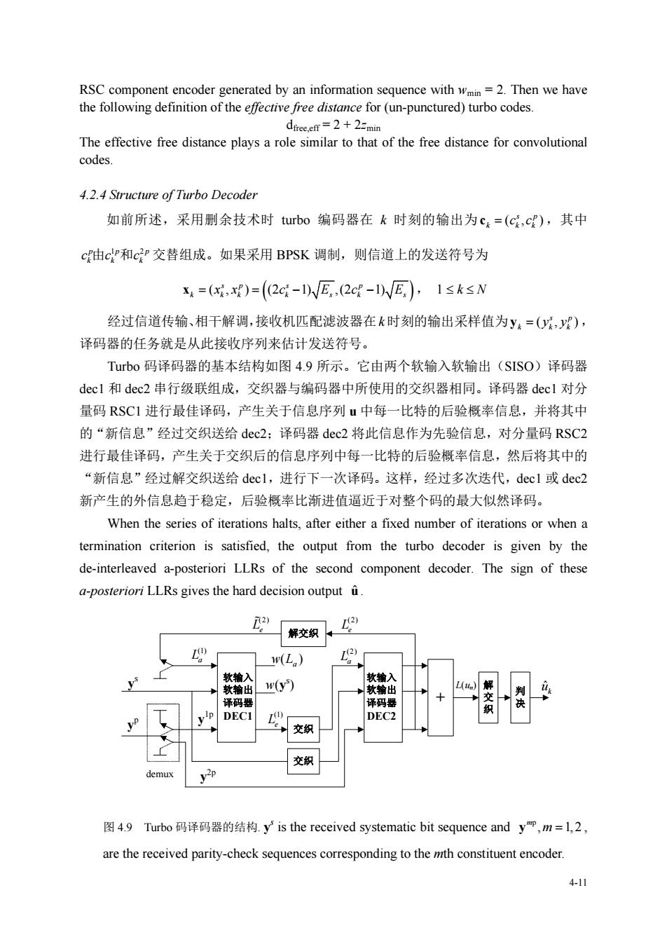
4-11 RSC component encoder generated by an information sequence with wmin = 2. Then we have the following definition of the effective free distance for (un-punctured) turbo codes. dfree,eff = 2 + 2zmin The effective free distance plays a role similar to that of the free distance for convolutional codes. 4.2.4 Structure of Turbo Decoder 如前所述,采用删余技术时 turbo 编码器在 k 时刻的输出为 (, ) s p k kk c c c ,其中 pp p 1 2 kk k cc c 由 和 交替组成。如果采用 BPSK 调制,则信道上的发送符号为 ( , ) (2 1) ,(2 1) sp s p k kk k s k s x x x c Ec E , 1 k N 经过信道传输、相干解调,接收机匹配滤波器在 k 时刻的输出采样值为 (, ) s p k kk y y y , 译码器的任务就是从此接收序列来估计发送符号。 Turbo 码译码器的基本结构如图 4.9 所示。它由两个软输入软输出(SISO)译码器 dec1 和 dec2 串行级联组成,交织器与编码器中所使用的交织器相同。译码器 dec1 对分 量码 RSC1 进行最佳译码,产生关于信息序列 u 中每一比特的后验概率信息,并将其中 的“新信息”经过交织送给 dec2;译码器 dec2 将此信息作为先验信息,对分量码 RSC2 进行最佳译码,产生关于交织后的信息序列中每一比特的后验概率信息,然后将其中的 “新信息”经过解交织送给 dec1,进行下一次译码。这样,经过多次迭代,dec1 或 dec2 新产生的外信息趋于稳定,后验概率比渐进值逼近于对整个码的最大似然译码。 When the series of iterations halts, after either a fixed number of iterations or when a termination criterion is satisfied, the output from the turbo decoder is given by the de-interleaved a-posteriori LLRs of the second component decoder. The sign of these a-posteriori LLRs gives the hard decision output u . 交织 解 交 织 软输入 软输出 译码器 DEC1 L(un) yp 交织 demux ys y1p y2p 解交织 + 判 决 w(ys ) 软输入 软输出 译码器 DEC2 (1) La (2) Le (1) Le ( ) w La k uˆ (2) Le (2) La 图 4.9 Turbo 码译码器的结构. ys is the received systematic bit sequence and p , 1,2 m y m , are the received parity-check sequences corresponding to the mth constituent encoder
下面我们对此迭代译码原理做一简要的讨论。假定tubo码译码器的接收序列为 y=(y',y),where y'is the received systematic bit sequence and y is the received parity-check sequence.冗余信息y经解复用后得到两个观测序列yP={P)和y2P={bP, 1≤k≤N,分别送给decl和dec2。这里,ym,m=lor2,is the noisy observation of if is not punctured;.otherwise,.setP=0(implying no observation obtained).于是,两 个软输出译码器的输入序列分别为: decl:y=(y',yP), dec2:y=(y',y) 为了使译码后的比特错误概率最小,根据最大后验概率(MAP)译码准则,tubo译码器的 最佳译码策略是,根据接收序列y计算后验概率(APP)P(u)=P(4:y",y2): MAP rule:arm(y) (4.2) 显然,式(4.2)的计算对于码长稍微长一点的码来说,计算复杂度太高。在tubo码 的译码方案中,巧妙地采用了一种次优译码规则,将y四和y2)分开考虑,由两个分量码 译码器分别计算后验概率P(4Iy",L)和P(4:Iy,Lg),然后通过decl和dec2之间 的多次迭代,使它们收敛于MAP译码的P(u:y",y2),从而达到逼近Shannon限的性 能。这里,和L为附加信息,其中L由decl提供,在dec2中用作先验信息:L 由dec2提供,在decl中用作先验信息。具体推导如下: P(u=uly'.y.y)=>P(uly'.y.y) 王p0产yIno =£pwmn0,ImP lyy") From distribution separation, Puly,yP)≈ΠPu.Iy',yP) 412
4-12 下面我们对此迭代译码原理做一简要的讨论。假定 turbo 码译码器的接收序列为 ( , ) s p y y y ,where ys is the received systematic bit sequence and p y is the received parity-check sequence. 冗余信息 p y 经解复用后得到两个观测序列 11 2 2 {} {} pp p p k k y y = 和= y y , 1 k N,分别送给 dec1 和 dec2。这里, p , 1 or 2 m k y m , is the noisy observation of mp k x if mp k x is not punctured; otherwise, set p 0 m k y (implying no observation obtained). 于是,两 个软输出译码器的输入序列分别为: dec1: (1) 1p (, ) s y yy , dec2: (2) 2p (, ) s y yy 为了使译码后的比特错误概率最小,根据最大后验概率(MAP)译码准则,turbo 译码器的 最佳译码策略是,根据接收序列 y 计算后验概率(APP) (1) (2) () | , Pu P u k k y y : MAP rule: 1 2 {0,1} ˆ arg max ( | , , ) s p p k k u u Pu u yy y (4.2) 显然,式(4.2)的计算对于码长稍微长一点的码来说,计算复杂度太高。在 turbo 码 的译码方案中,巧妙地采用了一种次优译码规则,将 (1) y 和 (2) y 分开考虑,由两个分量码 译码器分别计算后验概率 (1) (2) | , P uk e y L 和 (2) (1) | , P uk e y L ,然后通过 dec1 和 dec2 之间 的多次迭代,使它们收敛于 MAP 译码的 (1) (2) | , P uk y y ,从而达到逼近 Shannon 限的性 能。这里, (1) Le 和 (2) Le 为附加信息,其中 (1) Le 由 dec1 提供,在 dec2 中用作先验信息; (2) Le 由 dec2 提供,在 dec1 中用作先验信息。具体推导如下: 12 12 : ( | , , ) (| , , ) k s p p sp p k u u Pu u P u yy y u yy y 1 2 : ( , , | ) () k sp p u u p P u yy y u u 2 1 : ( | )( , | ) () k p sp u u pp P u y u y y u u 2 1 : ( |)(| , ) k p sp u u p P u y u u y y From distribution separation, 1 1 1 (| , ) ( | , ) N s p sp n n P Pu u yy yy
p(y'.ylu)P(u) Thus, P4=,y)xpwIp,yIP) Used as the priori probability for thedecoder Since the separation assumption destroyed optimality of the equation,the algorithm is iterated several times through the two decoders 需要说明的是,通过迭代译码提高编码方案性能的思想,早在60年代Gallager提 出的低密度校验码(LDPC)中己经萌芽]。在那里Gallager将信息分为内信息和外信 息两种,并指出只有外信息对迭代译码是有用的。但限于当时的实验条件与研究方法, 他没有给出迭代算法正确性的证明,只是通过一个例子说明了长的LDC码可以达到 BSC信道的容量。否则,信道编码理论的发展历史可能要被重新书写。 另外,既然只 有外信息可用于迭代,那么在迭代译码中,分量译码器之间的信息交 换应不相关,即要求交织器应最大程度地置乱原信息序列。 关于P(u,y",L2)和P(w,ly,)的求解,目前已有多种方法,它们构成了tubo 码的不同译码算法,我们将在后续章节中详细介绍。下面我们以BCJR的前向-后向MAP 软输出算法为例来讨论turbo码的译码。 4.3 Principle of Iterative Decoding Algorithm 4.3.1 Log Likelihood Ratios The concept of Log-Likelihood Ratios(LLRs)was shown by Robertson [to simplify the passing of information from one component decoder to the other in the iterative decoding of turbo codes,and so is now widely used in the turbo coding literature.Let be in GF(2) null e ement under the addition operation.The LLR oan别 (4.3) Here.P(denotes the probability that the random variable takeson the value Notice that the two possible values for the bit uare taken to be+1 and-1,rather than 0 and 1.This definition of the two values of a binary variable makes no conceptual difference,but it slightly simplifies the mathematics in the derivations which follow. Figure 4.10 shows how L(u)varies as the probability of =+1 varies.It can be seen from this figure that the sign of the LLRL()ofa bit is the hard decision,and the magnitude of the LLR gives the reliability of this decision(of how likely it is that the sign of the LLR gives the correct value of u.) 413
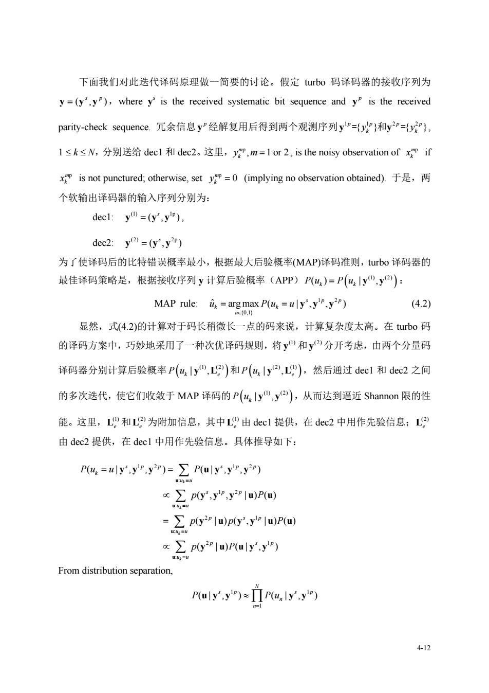
4-13 1 1 ( , | )( ) N s p n n n p u Pu y y Thus, 12 2 1 : 1 ( | , , ) ( |) ( , | )( ) k N sp p p sp k n n u u n Pu u p p u Pu u yy y y u yy Since the separation assumption destroyed optimality of the equation, the algorithm is iterated several times through the two decoders. 需要说明的是,通过迭代译码提高编码方案性能的思想,早在 60 年代 Gallager 提 出的低密度校验码(LDPC)中已经萌芽[?]。在那里 Gallager 将信息分为内信息和外信 息两种,并指出只有外信息对迭代译码是有用的。但限于当时的实验条件与研究方法, 他没有给出迭代算法正确性的证明,只是通过一个例子说明了长的 LDPC 码可以达到 BSC 信道的容量。否则,信道编码理论的发展历史可能要被重新书写。 另外,既然只有外信息可用于迭代,那么在迭代译码中,分量译码器之间的信息交 换应不相关,即要求交织器应最大程度地置乱原信息序列。 关于 (1) (2) | , P uk e y L 和 (2) (1) | , P uk e y L 的求解,目前已有多种方法,它们构成了 turbo 码的不同译码算法,我们将在后续章节中详细介绍。下面我们以 BCJR 的前向-后向 MAP 软输出算法为例来讨论 turbo 码的译码。 4.3 Principle of Iterative Decoding Algorithm 4.3.1 Log Likelihood Ratios The concept of Log-Likelihood Ratios (LLRs) was shown by Robertson [] to simplify the passing of information from one component decoder to the other in the iterative decoding of turbo codes, and so is now widely used in the turbo coding literature. Let u be in GF(2) with elements {+1, -1}, where ‘+1’ is the null element under the addition operation. The LLR or L-value of the binary variable u is defined to be ( 1) ( ) ln ( 1) P u L u P u (4.3) Here, P(u = i) denotes the probability that the random variable u takes on the value i. Notice that the two possible values for the bit u are taken to be +1 and -1, rather than 0 and 1. This definition of the two values of a binary variable makes no conceptual difference, but it slightly simplifies the mathematics in the derivations which follow. Figure 4.10 shows how L(u) varies as the probability of u=+1 varies. It can be seen from this figure that the sign of the LLR L(u) of a bit u is the hard decision, and the magnitude of the LLR gives the reliability of this decision (i.e., indication of how likely it is that the sign of the LLR gives the correct value of u.) Used as the priori probability for the 2nd decoder
0 0.1 0.2 0.3 0.4 P1 0.6 0.7 0.80.9 Figure 4.10 Log Likelihood Ratio L(u)versus the Probability of u=+1 For a data bit given the LLR L(),it is possible to calculate the probability that +1 or =-1.Noting that P(u=-1)=1-P(u=+1),and taking the exponent of both sides in (4.3)we have e4)=P4=+) 1-P(44=+l) P4:=+l)=+e4网-1+e网 and e-lm) P4,=-l)=1+e1+e Hence,we can write (e42) (4.4 e42 where Cdepends only on the LLR)and not on whetherisrt 414
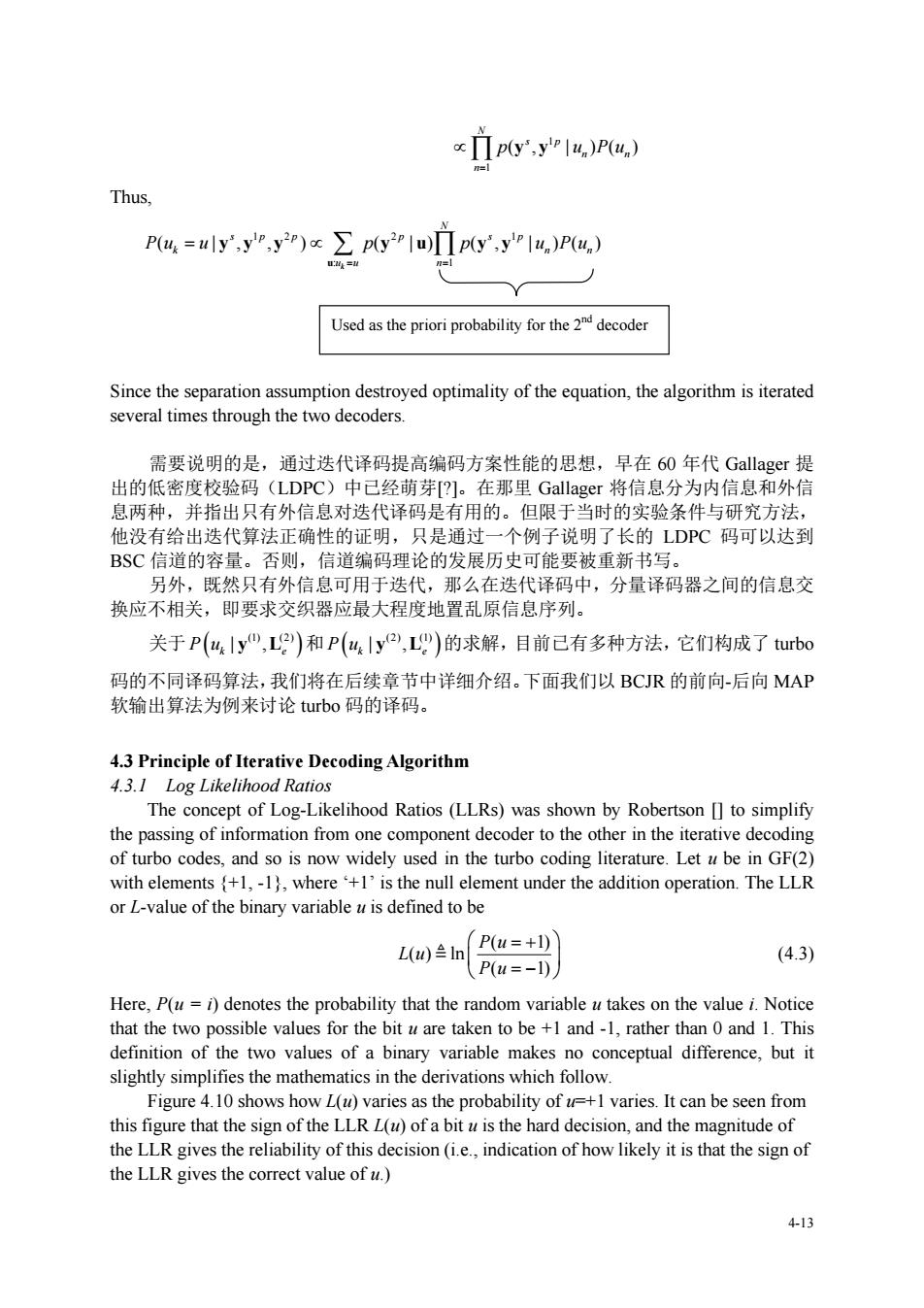
4-14 0 0.1 0.2 0.3 0.4 0.5 0.6 0.7 0.8 0.9 1 -8 -6 -4 -2 0 2 4 6 8 P(u=+1) L(u) Figure 4.10 Log Likelihood Ratio L(u) versus the Probability of u = +1 For a data bit uk, given the LLR L(uk), it is possible to calculate the probability that uk = +1 or uk = -1. Noting that ( 1) 1 ( 1) Pu Pu k k , and taking the exponent of both sides in (4.3) we have ( ) ( 1) 1 ( 1) L uk k k P u e P u so ( ) () () 1 ( 1) 1 1 k k k L u k Lu Lu e P u e e and ( ) () () 1 ( 1) 1 1 k k k L u k Lu Lu e P u e e Hence, we can write ( )/2 ( )/2 ( )/2 ( ) ( 1) 1 k k kk k L u Lu uLu k k L u e Pu e C e e (4.4) where ( )/2 ( ) 1 k k L u k L u e C e depends only on the LLR L(uk) and not on whether uk is +1 or –1, so it
can be treated as a constant.Eq.(4.4)can also be expressed as ±L(2 Pu:=圳=e4+e We define the soft bit()as the expectation of u.From the discussion above,we have A(4)=曰4] =(+)P(4=+)+(-1)P(4=-I) =tanhL() 2 If P()is a random variable in the range of (1),then()is a random variable(r.v.)in the range (-1,+1).For two binary random variables u and uz,their GF(2)addition u transforms into uu Since Eluu]=E[u ]E[u]=()(u),the LLR of the sum L(4⊕42)equals tanh-tanh.tanh=L(t )L(u 2 abbreviated by the boxplus operation This relation is often used in the decoding of LDPC codes,and appeared in the following form. 定义(Box-PIus运算):对于两个二元独立随机变量u和y,它们的box-plus运算定义 为 L0②Lm)=Lu田p=logP引=bg。+e4 * As well as the LLR L()based on the unconditional probabilities P(=),we are also interested in LLRs based on conditional probabilities.For example,we often use the conditional LLRs based on the probability that the receiver's matched filter output would be y&given that the corresponding transmitted bitx=+1 or-1.This conditional LLR,denoted by P(yx).is defined as w (4.5) If we assume that xa is transmitted over the(possibly fading)AWGN channel using BPSK 4-15
4-15 can be treated as a constant. Eq. (4.4) can also be expressed as ( )/2 ( )/2 ( )/2 ( 1) k k k L u k Lu Lu e P u e e We define the soft bit ( ) k u as the expectation of uk. From the discussion above, we have () [] k k u u E ( 1) ( 1) ( 1) ( 1) Pu Pu k k ( ) tanh 2 L uk If P(uk) is a random variable in the range of (0, 1), then ( ) k u is a random variable (r.v.) in the range (-1, +1). For two binary random variables u1 and u2, their GF(2) addition 1 2 u u transforms into 1 2 u u . Since 12 1 2 1 2 Eu u Eu Eu u u [ ] [] [] () () , the LLR of the sum L 1 2 u u equals 1 1 2 1 2 () () 2 tanh tanh tanh ( ) ( ) 2 2 Lu Lu Lu Lu abbreviated by the boxplus operation . This relation is often used in the decoding of LDPC codes, and appeared in the following form. 定义(Box-Plus 运算):对于两个二元独立随机变量 u 和 v,它们的 box-plus 运算定义 为 () () () () ( 0) 1 ( ) ( ) ( ) log log ( 1) Lu Lv Lu Lv Pu v e Lu Lv Lu v Pu v e e As well as the LLR L(uk) based on the unconditional probabilities ( 1) P uk , we are also interested in LLRs based on conditional probabilities. For example, we often use the conditional LLRs based on the probability that the receiver’s matched filter output would be yk given that the corresponding transmitted bit 1 or 1 k x . This conditional LLR, denoted by (|) Py x k k , is defined as ( | 1) ( | ) ln ( | 1) k k k k k k Py x Ly x Py x (4.5) If we assume that xk is transmitted over the (possibly fading) AWGN channel using BPSK