21/88 3.2.3 Some Basic Statistics(统计学) 4.Perfect Gaussian Distribution For a perfect Gaussian distribution,it can be shown that 68%of the readings lie within±1aofμ 95%of the readings lie within±2aofμ .(3.9) 99.7%of the readings lie within±3aofμ Question:for the pressure gage readings(u=10.11 and o=0.14), if sufficient readings were taken,then how many readings can fall within±0.42of10.11? Answer:99.7% 22/88 3.2.3 Some Basic Statistics(统计学) 4.Perfect Gaussian Distribution (continued) The purpose of the calibration is to convert instrument readings into estimates of the true value. For example,a calibrated gage(X=10.11,S=0.14)is used to measure an unknown pressure and the gage happened to read as 10.11,we would say: Our best estimation of the true pressure is 10.00(why this is the best?); But this value is uncertain; -The uncertainty cannot be removed but we can quantify(量化,定量描述)it. We are 68%sure the true value is within +0.14 of 10.00,95%sure it is within±0.28,and99.7%sure it is within±0.42. The basic precision index is s(0.14),but it has been common practice to quote the imprecision(不准确度)as士3s
For a perfect Gaussian distribution, it can be shown that : 68% of the readings lie within ±1σ of μ 95% of the readings lie within ±2σ of μ … (3.9) 99.7% of the readings lie within ±3σ of μ Question: for the pressure gage readings (μ=10.11 and σ=0.14), if sufficient readings were taken, then how many readings can fall within ±0.42 of 10.11? Answer: 99.7% 3.2.3 Some Basic Statistics(统计学) 4. Perfect Gaussian Distribution 21/88 The purpose of the calibration is to convert instrument readings into estimates of the true value. For example, a calibrated gage (ܺ=10.11, S=0.14) is used to measure an unknown pressure and the gage happened to read as 10.11, we would say : - Our best estimation of the true pressure is 10.00 (why this is the best?); - But this value is uncertain; - The uncertainty cannot be removed but we can quantify(量化,定量描述) it. - We are 68% sure the true value is within ±0.14 of 10.00, 95% sure it is within ±0.28, and 99.7% sure it is within ±0.42. - The basic precision index is s(0.14), but it has been common practice to quote the imprecision(不准确度) as ±3s. 3.2.3 Some Basic Statistics(统计学) 4. Perfect Gaussian Distribution (continued) 22/88
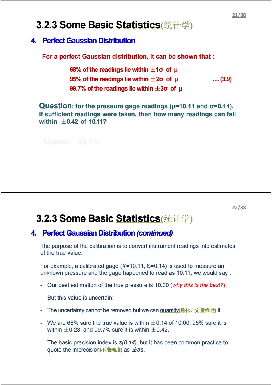
23/88 3.2.3 Some Basic Statistics(统计学) 4.Perfect Gaussian Distribution(continued) ±3 s imprecision Reading True value Bias I 1 9.58 10.0010.11 10.42p,kPa Figure 3.3b Pressure-Gage Calibration Data Since most engineering samples are relatively small,it was decided that quoting uncertainty bands at the 95%level of confidence was more realistic than using the older 99.7%criterion.(why?) 24/88 3.2.4 Least-Squares Calibration Curves 1.Basic Knowledge In an actual instrument calibration,the true value is varied over some range,causing the measured value also to vary over a range; The measured values and true values can be displayed as scattered points in a 2D graph. Criterion can be defined to best fits the scattered points into an averaged calibration curve (fitted curve). Least-squares criterion is the most common one,which minimizes the sum of the squares of the vertical deviations of the data points from the fitted curve
Figure 3.3b Pressure - Gage Calibration Data Since most engineering samples are relatively small, it was decided that quoting uncertainty bands at the 95% level of confidence was more realistic than using the older 99.7% criterion. (why?) 3.2.3 Some Basic Statistics(统计学) 4. Perfect Gaussian Distribution (continued) 23/88 3.2.4 Least-Squares Calibration Curves 1. Basic Knowledge In an actual instrument calibration, the true value is varied over some range, causing the measured value also to vary over a range; The measured values and true values can be displayed as scattered points in a 2D graph. Criterion can be defined to best fits the scattered points into an averaged calibration curve (fitted curve). Least-squares criterion is the most common one, which minimizes the sum of the squares of the vertical deviations of the data points from the fitted curve. 24/88

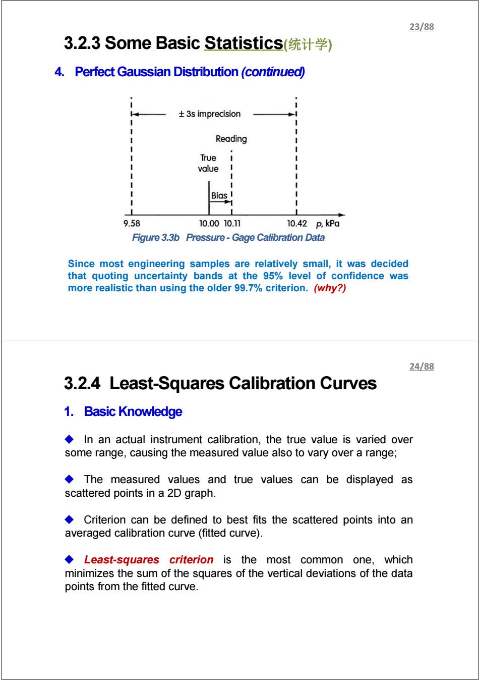
25/88 3.2.4 Least-Squares Calibration Curves 2.Fitted Straight Line Indicoted pressure o-Increasing true pressure k炉a Increasing Decreosing -Decreasing true pressure 0.000 -1.12 -0.69 .000 0.21 0.42 Instrument Bias:the predicted 2.000 118 1.65 difference on average between the 5.000 6.000 5.26 measurement and the true value. 7.000 6.59 8.000 7.73 9.000 8.68 9.10 10.000 9.80 10.20 ±3 s uncertainty limits ±0.58 imprecision Least-squares fitted line Bias 4=1.0829-0.847 (-0.46) Acceleration =0 Vibration level =0- Ambient temperature =20±1C Pressure 4.20 4.32 4.78 536 10 Reading Best estimate u ure.kPo of true value (b) Figure 3.10 Pressure Gage Calibration 26/88 3.2.4 Least-Squares Calibration Curves 2.Fitted Straight Line (continued) 9o mqi +b .…(3.11) qo 2 output quantity (dependent variable) ..(3.12) qi 2 input quantity (independent variable) .(3.13) m≌slope of line .(3.14) bintercept of line on vertical axis ..(3.15) N∑q:9。-(②q9o 1n= (3.16 N∑qi-(②q2 b=9.2g-②49q (3.17) N∑qi-(②q2 NA total number of data points (3.18)
3.2.4 Least-Squares Calibration Curves 2. Fitted Straight Line Figure 3.10 Pressure Gage Calibration Instrument Bias : the predicted difference on average between the measurement and the true value. 25/88 3.2.4 Least-Squares Calibration Curves 2. Fitted Straight Line (continued) (12.3ܾ݈݅ܽ݁) … (ݎܽݒ ݐ݊݁݀݊݁݁݀) ݕݐ݅ݐ݊ܽݑݍ output ≜ ݍ (11.3 + ܾ … (ݍ݉ = ݍ (13.3ܾ݈݅ܽ݁) … (ݎܽݒ ݐ݊݁݀݊݁݁݀݊݅) ݕݐ݅ݐ݊ܽݑݍ put ≜ ݅݊ݍ (14.3݂ ݈݅݊݁ … ( ݈݁ݏ ≜ ݉ (15.3 … (ݏ݅ݔܽ ݈ܽܿ݅ݐݎ݁ݒ ݊ ݈݁݊݅ ݂ ݐ݁ܿݎ݁ݐ݊݅ ≜ ܾ 26/88
27/88 3.2.4 Least-Squares Calibration Curves 2.Fitted Straight Line(continued Least-Squares Calibration Curves.xlsx The total error of a measurement process can be decomposed into two parts:the bias and the imprecision. Once the instrument has been calibrated,the bias error can be removed via calibration,and the only remaining error is that due to imprecision. The bias error is called the systematic error;the error due to imprecision is called random error. Calibration is the process of removing bias and defining imprecision numerically Accuracy is often quoted as a percentage figure based on the full-scale reading of the instrument. 28/88 3.2.5 Calibration Accuracy versus Installed Accuracy 1.Basic Knowledge When the instrument is used,it is rarely possible to maintain that carefully controlled environment in experimental apparatus. The measurement error (bias and imprecision)must be re-evaluated, taking into account,as best possible,the deviation of the measurement conditions from the calibration conditions. The re-evaluation is usually not straightforward.Judgment and past experience(rather than "scientific"calculation)is often necessary. The unknown bias in the measurement situation (as contract with calibration) is treated as a random effect rather than as a systematic. Bias limit,is defined as the range of values within which we feel that the actual bias will be found 95%of the time.The 95%value was chosen to make it consistent with the 95%confidence limit for the imprecision
Least-Squares Calibration Curves.xlsx The total error of a measurement process can be decomposed into two parts: the bias and the imprecision. Once the instrument has been calibrated, the bias error can be removed via calibration, and the only remaining error is that due to imprecision. The bias error is called the systematic error; the error due to imprecision is called random error. Calibration is the process of removing bias and defining imprecision numerically Accuracy is often quoted as a percentage figure based on the full-scale reading of the instrument. 3.2.4 Least-Squares Calibration Curves 2. Fitted Straight Line (continued) 27/88 3.2.5 Calibration Accuracy versus Installed Accuracy 1. Basic Knowledge When the instrument is used, it is rarely possible to maintain that carefully controlled environment in experimental apparatus. The measurement error (bias and imprecision) must be re-evaluated, taking into account, as best possible, the deviation of the measurement conditions from the calibration conditions. The re-evaluation is usually not straightforward. Judgment and past experience (rather than “scientific” calculation) is often necessary. The unknown bias in the measurement situation (as contract with calibration) is treated as a random effect rather than as a systematic. Bias limit, is defined as the range of values within which we feel that the actual bias will be found 95% of the time. The 95% value was chosen to make it consistent with the 95% confidence limit for the imprecision. 28/88
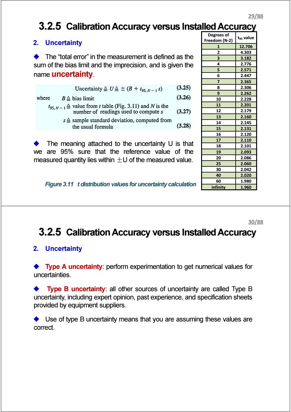
29/88 3.2.5 Calibration Accuracy versus Installed Accuracy Degrees of 2.Uncertainty Freedom(N-2) t9s value 12.706 2 4.303 The"total error"in the measurement is defined as the 心 3.182 sum of the bias limit and the imprecision,and is given the 4 2.776 2.571 name uncertainty. 6 2.447 7 2.365 UncertaintyU (B t95.N-1) (3.25) 8 2.306 9 2.262 where B≌bias limit (3.20 10 2.228 19s.N-1A value from t table (Fig.3.11)and N is the 11 2.201 number of readings used to compute s (3.27) 12 2.179 13 2.160 sA sample standard deviation,computed from 14 2.145 the usual formula (3.28) 15 2.131 16 2.120 17 2.110 The meaning attached to the uncertainty U is that 18 2.101 we are 95%sure that the reference value of the 19 2.093 measured quantity lies within +U of the measured value. 20 2.086 25 2.060 30 2.042 40 2.020 60 1.980 Figure 3.11 t distribution values for uncertainty calculation infinity 1.960 30/88 3.2.5 Calibration Accuracy versus Installed Accuracy 2.Uncertainty Type A uncertainty:perform experimentation to get numerical values for uncertainties. Type B uncertainty:all other sources of uncertainty are called Type B uncertainty,including expert opinion,past experience,and specification sheets provided by equipment suppliers. Use of type B uncertainty means that you are assuming these values are correct
3.2.5 Calibration Accuracy versus Installed Accuracy 2. Uncertainty The “total error” in the measurement is defined as the sum of the bias limit and the imprecision, and is given the name uncertainty. The meaning attached to the uncertainty U is that we are 95% sure that the reference value of the measured quantity lies within ±U of the measured value. Degrees of Freedom (N-2) t95 value 1 12.706 2 4.303 3 3.182 4 2.776 5 2.571 6 2.447 7 2.365 8 2.306 9 2.262 10 2.228 11 2.201 12 2.179 13 2.160 14 2.145 15 2.131 16 2.120 17 2.110 18 2.101 19 2.093 20 2.086 25 2.060 30 2.042 40 2.020 60 1.980 infinity 1.960 Figure 3.11 t distribution values for uncertainty calculation 29/88 3.2.5 Calibration Accuracy versus Installed Accuracy 2. Uncertainty Type A uncertainty: perform experimentation to get numerical values for uncertainties. Type B uncertainty: all other sources of uncertainty are called Type B uncertainty, including expert opinion, past experience, and specification sheets provided by equipment suppliers. Use of type B uncertainty means that you are assuming these values are correct. 30/88