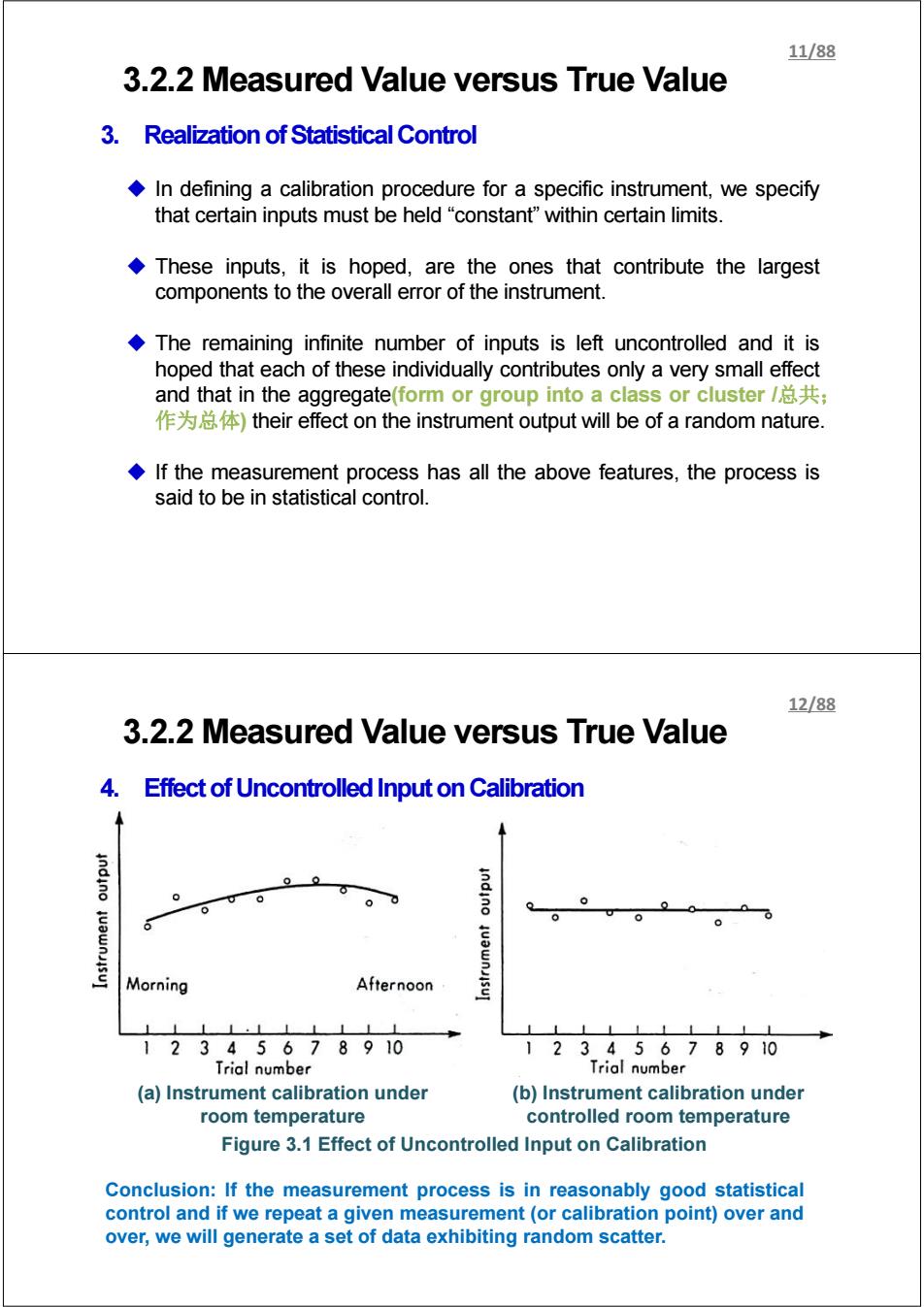
11/88 3.2.2 Measured Value versus True Value 3.Realization of Statistical Control In defining a calibration procedure for a specific instrument,we specify that certain inputs must be held "constant"within certain limits. These inputs,it is hoped,are the ones that contribute the largest components to the overall error of the instrument. The remaining infinite number of inputs is left uncontrolled and it is hoped that each of these individually contributes only a very small effect and that in the aggregate(form or group into a class or cluster总共; 作为总体)their effect on the instrument output will be of a random nature. If the measurement process has all the above features,the process is said to be in statistical control. 12/88 3.2.2 Measured Value versus True Value 4.Effect of Uncontrolled Input on Calibration indino 0 indino 6 Morning Afternoon 111 11 12345678910 12345678910 Trial number Trial number (a)Instrument calibration under (b)Instrument calibration under room temperature controlled room temperature Figure 3.1 Effect of Uncontrolled Input on Calibration Conclusion:If the measurement process is in reasonably good statistical control and if we repeat a given measurement (or calibration point)over and over,we will generate a set of data exhibiting random scatter
3.2.2 Measured Value versus True Value 3. Realization of Statistical Control In defining a calibration procedure for a specific instrument, we specify that certain inputs must be held “constant” within certain limits. These inputs, it is hoped, are the ones that contribute the largest components to the overall error of the instrument. The remaining infinite number of inputs is left uncontrolled and it is hoped that each of these individually contributes only a very small effect and that in the aggregate(form or group into a class or cluster /总共; 作为总体) their effect on the instrument output will be of a random nature. If the measurement process has all the above features, the process is said to be in statistical control. 11/88 3.2.2 Measured Value versus True Value 4. Effect of Uncontrolled Input on Calibration (a) Instrument calibration under room temperature (b) Instrument calibration under controlled room temperature Figure 3.1 Effect of Uncontrolled Input on Calibration Conclusion: If the measurement process is in reasonably good statistical control and if we repeat a given measurement (or calibration point) over and over, we will generate a set of data exhibiting random scatter. 12/88

13/88 3.2.2 Measured Value versus True Value 5.Calibration and Application Conditions Desired Input: 习Pressure Other possible Inputs: Temperature,acceleration,vibration,etc. It is important to carefully consider the relationship between the calibration conditions and the actual application conditions. Pointer Fluid Piston Piston rod Spring Linkage and scale Primary Vorioble- Motion Variable- Motion Dato- Pressure Force sensing conversion tronsmission conversion Measured element element element element element element Figure 3.2 Pressure Gauge 14/88 3.2.3 Some Basic Statistics(统计学) 1.Probability Cumulative Probability Trial Number Scale Reading(kPa) 1 10.20 True Pressure (Reference Value)=10+.001kPa 2 10.20 Ambient Temperature=20±1℃ 3 10.26 Acceleration=0 Vibration=0 4 10.20 5 10.22 6 10.13 7 9.97 8 10.12 9 10.09 9.809.85g909.9510001005101010.5102010.25103010350.4010.4510.50 scale reading.kPa 10 9.90 Distribution of Data 11 10.05 f(x)=Z 12 10.17 13 10.42 14 10.21 F(x) Probability Distribution 15 10.23 1.0 16 10.11 17 9.98 18 10.10 Cumulative Probability Distribution 19 10.04 Pressure-Gage Calibration Data 20 9.81
3.2.2 Measured Value versus True Value 5. Calibration and Application Conditions Desired Input: Pressure Other possible Inputs: Temperature, acceleration, vibration, etc. Figure 3.2 Pressure Gauge It is important to carefully consider the relationship between the calibration conditions and the actual application conditions. 13/88 Cumulative Probability Distribution Distribution of Data 3.2.3 Some Basic Statistics(统计学) 1. Probability & Cumulative Probability Trial Number Scale Reading(kPa) 1 10.20 2 10.20 3 10.26 4 10.20 5 10.22 6 10.13 7 9.97 8 10.12 9 10.09 10 9.90 11 10.05 12 10.17 13 10.42 14 10.21 15 10.23 16 10.11 17 9.98 18 10.10 19 10.04 20 9.81 TruePressure(Reference Value) = 10±.001kPa Ambient Temperature = 20±1℃ Acceleration = 0 Vibration = 0 Pressure - Gage Calibration Data Probability Distribution 14/88
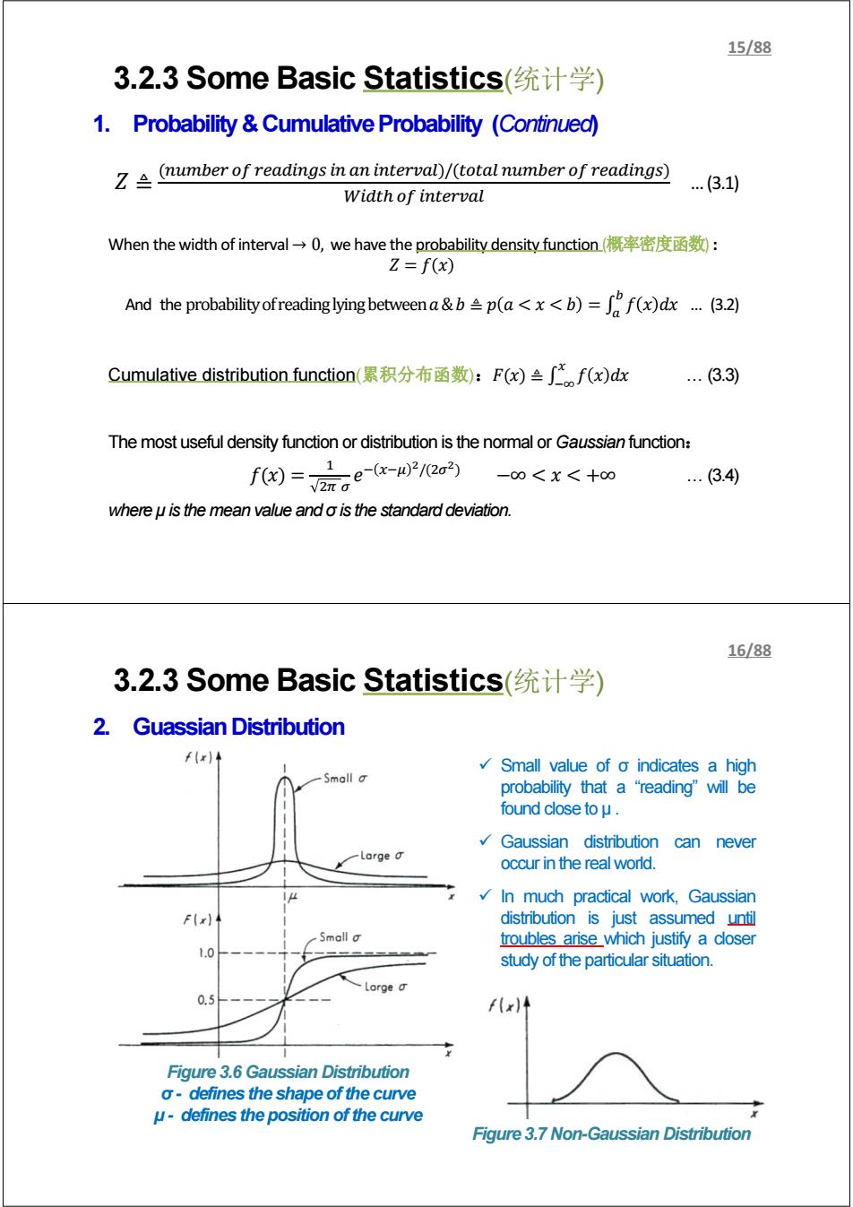
15/88 3.2.3 Some Basic Statistics(统计学) 1.Probability Cumulative Probability (Continued) mumber of readings in an interval)/(total number of readings) .(3.1) Width of interval When the width of interval-→O,we have the probability density function概率密度函数: Z=f(x) And the probabilityofreadinglying betweena&p(a=f(x)dx(3.2) Cumulative distribution function(累积分布函数):F(x)兰∫nf(x)dce ..(3.3) The most useful density function or distribution is the normal or Gaussian function: f0)=点aew-0/的 -0<X<+00 .(3.4) where u is the mean value and o is the standard deviation. 16/88 3.2.3 Some Basic Statistics(统计学) 2.Guassian Distribution ( Small value of o indicates a high Small probability that a“reading”wlbe found close to u. Gaussian distribution can never Large occur in the real world. In much practical work,Gaussian distribution is just assumed until Smallo troubles arise which justify a closer 1.0 study of the particular situation. 0.5 Figure 3.6 Gaussian Distribution o-defines the shape of the curve u-defines the position of the curve Figure 3.7 Non-Gaussian Distribution
ܼ ≜ (௨ ௗ௦ ௧௩)/(௧௧ ௨ ௗ௦) ௐௗ௧ ௧௩ … (3.1) When the width of interval → 0, we have the probability density function (概率密度函数) : ݔ ݂=ܼ ௫ ݔ݀ ݔ ݂ ≜ (ݔ)ܨ:(累积分布函数(function distribution Cumulative ିஶ … (3.3) The most useful density function or distribution is the normal or Gaussian function: ଵ) = ݔ)݂ ଶగ ఙ ݁ି ௫ିఓ మ/(ଶఙమ) −∞ < ݔ) ... ∞+ > 3.4) where μ is the mean value and σ is the standard deviation. And the probability of reading lying between ܽ & ܾ ≜ >ܽ ݔ = ܾ> ݂ ݔ݀ ݔ … (3.2) 3.2.3 Some Basic Statistics(统计学) 1. Probability & Cumulative Probability (Continued) 15/88 Figure 3.6 Gaussian Distribution σ - defines the shape of the curve μ - defines the position of the curve Figure 3.7 Non-Gaussian Distribution 9 Small value of σ indicates a high probability that a “reading” will be found close to μ . 9 Gaussian distribution can never occur in the real world. 9 In much practical work, Gaussian distribution is just assumed until troubles arise which justify a closer study of the particular situation. 3.2.3 Some Basic Statistics(统计学) 2. GuassianDistribution 16/88
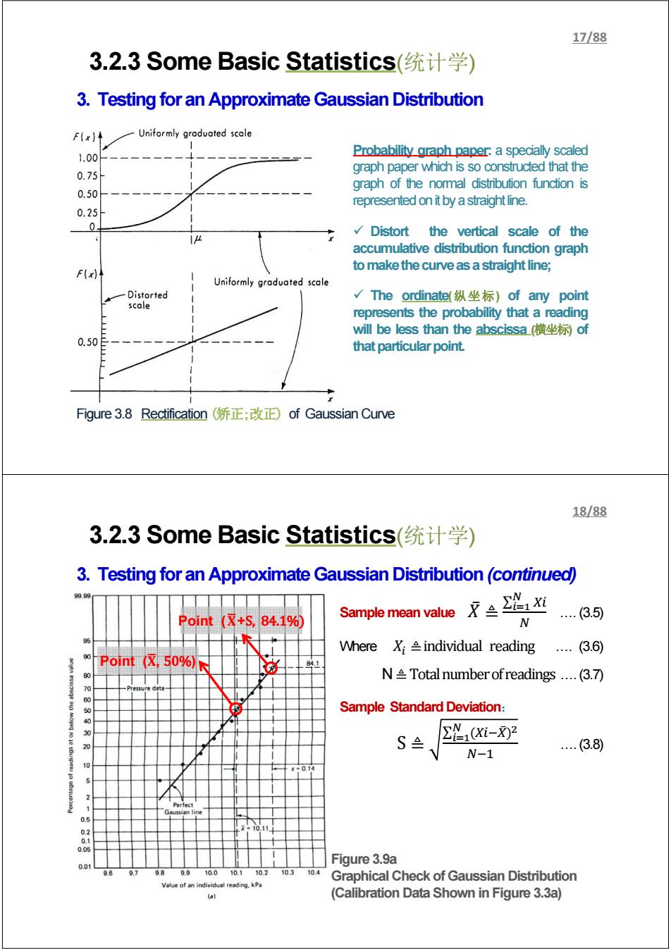
17/88 3.2.3 Some Basic Statistics(统计学) 3.Testing for an Approximate Gaussian Distribution FIx)↑ Uniformly graduated scale 1.00 Probability graph paper:a specially scaled 0.75 graph paper which is so constructed that the graph of the normal distribution function is 0.50 represented on it by a straight line. 0.25 0 Distort the vertical scale of the accumulative distribution function graph to make the curve as a straight line; F(x) Uniformly graduated scale Distorted √The ordinate(纵坐标)of any point scale represents the probability that a reading will be less than the abscissa横坐标of 0.50 that particular point. Figure 3.8 Rectification(矫正;改正)of Gaussian Curve 18/88 3.2.3 Some Basic Statistics(统计学) 3.Testing for an Approximate Gaussian Distribution(continued) Point(☒+S,84.1% Sample mean value京兰2&i N (3.5) Where X;individual reading ..(3.6) .0 Point(区,50%N N Total number ofreadings ...(3.7) Sample Standard Deviation: 30 S (Xi-X)2 20 ..(3.8) N-1 014 0.01 Figure 3.9a 96 97 98 9.9 10.0 10.1 10.2 10.3 10.4 Graphical Check of Gaussian Distribution Value of an individual reading.kPa (ol (Calibration Data Shown in Figure 3.3a)
3.2.3 Some Basic Statistics(统计学) 3. Testing for an Approximate Gaussian Distribution Figure 3.8 Rectification (矫正;改正) of Gaussian Curve Probability graph paper: a specially scaled graph paper which is so constructed that the graph of the normal distribution function is representedonitbyastraightline. 9 Distort the vertical scale of the accumulative distribution function graph tomakethecurveasastraightline; 9 The ordinate(纵坐标) of any point represents the probability that a reading will be less than the abscissa (横坐标) of thatparticularpoint. 17/88 Figure 3.9a Graphical Check of Gaussian Distribution (Calibration Data Shown in Figure 3.3a) Sample mean value ܺ̅≜ ∑ ಿ సభ ே …. (3.5) Where ܺ ≜ individual reading …. (3.6) N ≜ Total number of readings …. (3.7) Sample Standard Deviation: S ≜ ∑ (ି̅ ) ಿ మ సభ ேିଵ …. (3.8) Point (܆ഥ, 50%) Point (܆ഥ+S, 84.1%) 3.2.3 Some Basic Statistics(统计学) 3. Testing for an Approximate Gaussian Distribution (continued) 18/88
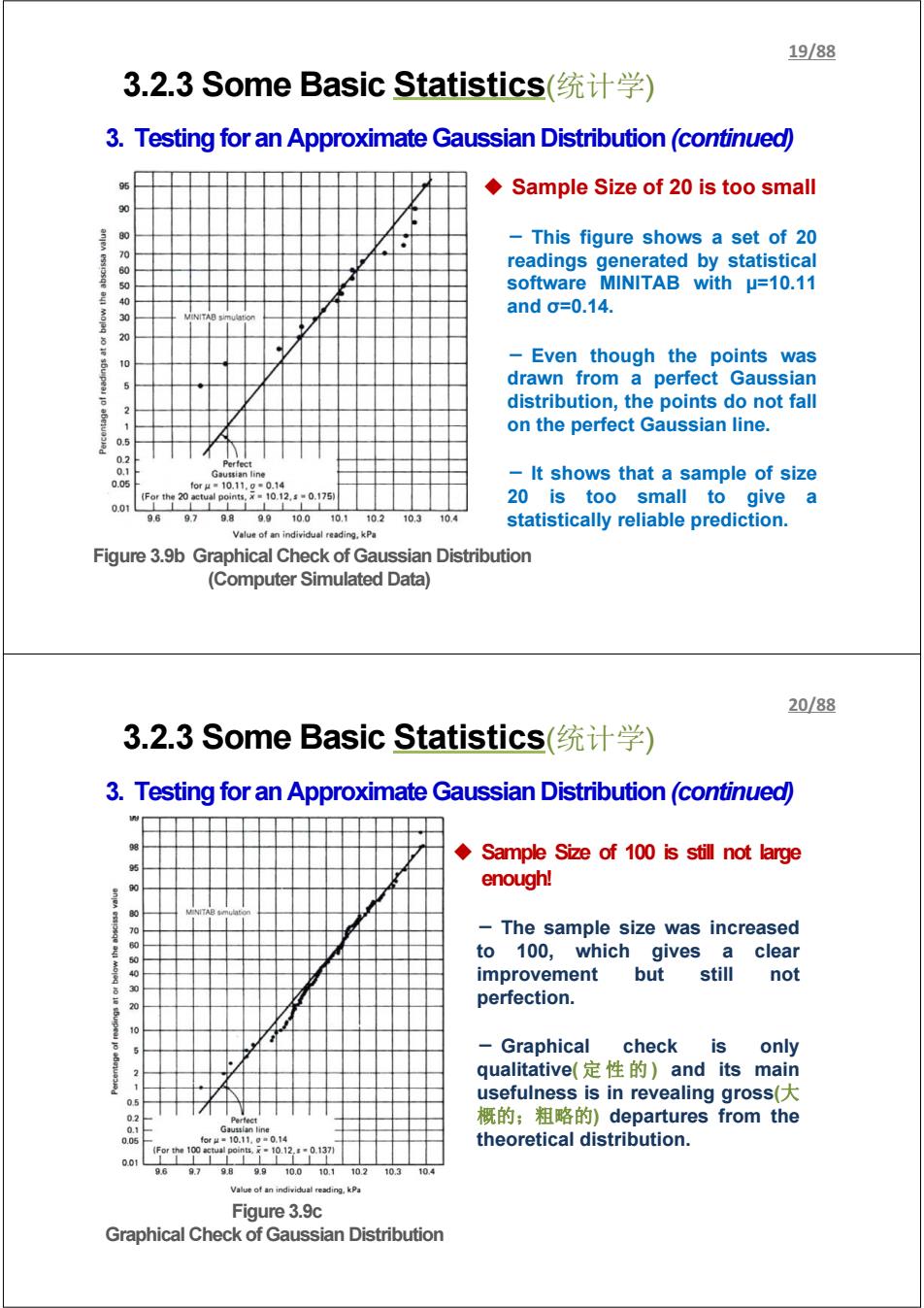
19/88 3.2.3 Some Basic Statistics(统计学) 3.Testing for an Approximate Gaussian Distribution (continued) Sample Size of 20 is too small 90 This figure shows a set of 20 70 60 readings generated by statistical 50 software MINITAB with u=10.11 and0=0.14. 3 VINITAB simu -Even though the points was drawn from a perfect Gaussian 5 distribution,the points do not fall on the perfect Gaussian line. 05 0.2 Perfect 0.1 Gaussian line 0.05 It shows that a sample of size for4=10.11.9=0.14 20 is too small to give a 0.01L 969.79.89.910.010.110.210.3 10.4 statistically reliable prediction. Value of an individual reading.kPa Figure 3.9b Graphical Check of Gaussian Distribution (Computer Simulated Data) 20/88 3.2.3 Some Basic Statistics(统计学) 3.Testing for an Approximate Gaussian Distribution(continued) Sample Size of 100 is still not large enough! 3 70 The sample size was increased to 100,which gives a clear 4 improvement but still not 20 perfection. 100 Graphical check is only qualitative(定性的)and its main usefulness is in revealing gross( 3 概的;粗略的)departures from the 01 Gaussian line 0.0 foeh-10.11.9m0.14 theoretical distribution. 001 96 9.7989910.0101102103 Value of an individual reading.kPa Figure 3.9c Graphical Check of Gaussian Distribution
Figure 3.9b Graphical Check of Gaussian Distribution (Computer Simulated Data) Sample Size of 20 is too small - This figure shows a set of 20 readings generated by statistical software MINITAB with μ=10.11 and σ=0.14. - Even though the points was drawn from a perfect Gaussian distribution, the points do not fall on the perfect Gaussian line. - It shows that a sample of size 20 is too small to give a statistically reliable prediction. 3.2.3 Some Basic Statistics(统计学) 3. Testing for an Approximate Gaussian Distribution (continued) 19/88 Figure 3.9c Graphical Check of Gaussian Distribution Sample Size of 100 is still not large enough! - The sample size was increased to 100, which gives a clear improvement but still not perfection. - Graphical check is only qualitative( 定性的 ) and its main usefulness is in revealing gross(大 概的;粗略的) departures from the theoretical distribution. 3.2.3 Some Basic Statistics(统计学) 3. Testing for an Approximate Gaussian Distribution (continued) 20/88