w=H”,ifM<N HH,ifM≥N This implies that det(I -W)=0 (8.9) The m nonzero eigenvalues of W. Am, can be calculated by finding the roots of ()The non-egativequre root of the of Ware lso referred to values of H. Substituting (8.6)into (8.1),we have y=UAV"x+n Let y=U"y,=V"x,n=U"n.Note that U and V are invertible,and n have the same distribution (ie.,zero-mean Gaussian with i.i.d.real and imaginary parts),and E[]=E[x"x].Thus the original channel defined in (8.1)is equivalent to the channel y=Ai+i (8.10) where A=diag(V万,V,√,0,0)with√,i=l,2,m denoting the non-zero singular values of H.The equivalence is summarized in Fig.8.2.From (8.10),we obtain for signal 立=V月元+元,1≤i≤m 元=元,m+1sisM (8.11) It is seen that received componentsi>m,do not depend on the transmitted signal.On the other hand,received componentsi=1,2,.m depend only the transmitted component ,Thus the equivalent MIMO channel in (8.10)can be considered as consisting of m uncoupled parallel Gaussian sub-channels.Specifically, If N>M (8.11)indicates that there will be at most M non-zero attenuation subchannels in the equivalent MIMO channel.See Fig.8.3 If N.there will be at most N non-zero attenuation subchannels in the equivalent MIMO channel
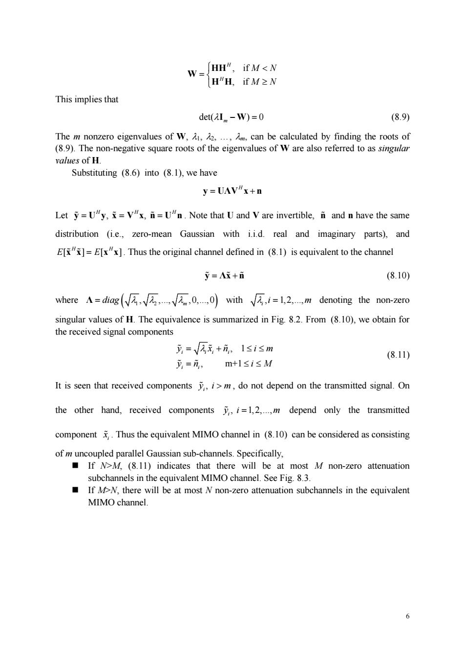
6 , if , if H H M N M N HH W H H This implies that det( ) 0 I W m (8.9) The m nonzero eigenvalues of W, 1, 2, ., m, can be calculated by finding the roots of (8.9). The non-negative square roots of the eigenvalues of W are also referred to as singular values of H. Substituting (8.6) into (8.1), we have H y U ΛVx n Let , , HHH y U y x Vxn Un . Note that U and V are invertible, n and n have the same distribution (i.e., zero-mean Gaussian with i.i.d. real and imaginary parts), and [][] H H E E xx xx . Thus the original channel defined in (8.1) is equivalent to the channel y Λx n (8.10) where 1 2 , ,., ,0,.,0 m Λ diag with , 1,2,., i i m denoting the non-zero singular values of H. The equivalence is summarized in Fig. 8.2. From (8.10), we obtain for the received signal components , 1 , m+1 i ii i i i y x n im y n iM (8.11) It is seen that received components , i y i m , do not depend on the transmitted signal. On the other hand, received components , 1,2,., i y i m depend only the transmitted component i x . Thus the equivalent MIMO channel in (8.10) can be considered as consisting of m uncoupled parallel Gaussian sub-channels. Specifically, If N>M, (8.11) indicates that there will be at most M non-zero attenuation subchannels in the equivalent MIMO channel. See Fig. 8.3. If M>N, there will be at most N non-zero attenuation subchannels in the equivalent MIMO channel
日 channel H Figure 8.2 Converting the MIMO channel into a parallel channel through the SVD. X r Xog'I 0 0 Fig.8.3 Block diagram of an equivalent MIMO channel for N>M With the above model (parallel orthogonal channels),the fundamental capacity of an MIMO channel can be cale ated in terms of the positive eigenvalues of the matrix HHas follows 8.3.2 Channel Known to the Transmitter When the perfect channel knowledge is available at both the transmitter and the receiver, the transmitter according to the Substituting the matrix SVD (8.6)into (8.5)and using properties of unitary matrices,we get the MIMO capacity with CSIT and CSIR as 7
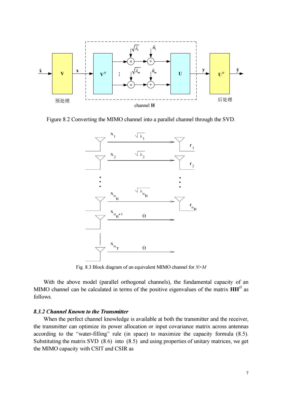
7 V U x H V . + + H U 1 m 1 n mn y 预处理 后处理 channel H x y Figure 8.2 Converting the MIMO channel into a parallel channel through the SVD. Fig. 8.3 Block diagram of an equivalent MIMO channel for N>M With the above model (parallel orthogonal channels), the fundamental capacity of an MIMO channel can be calculated in terms of the positive eigenvalues of the matrix HHH as follows. 8.3.2 Channel Known to the Transmitter When the perfect channel knowledge is available at both the transmitter and the receiver, the transmitter can optimize its power allocation or input covariance matrix across antennas according to the “water-filling” rule (in space) to maximize the capacity formula (8.5). Substituting the matrix SVD (8.6) into (8.5) and using properties of unitary matrices, we get the MIMO capacity with CSIT and CSIR as
C=ea+元K,刃》 =路2e1+光) whereP is the transmit power in the th sub-channel.Solving the optimiation leads toa water-filling power allocation over the parallel channels.The power allocated to channel i. 1sism,is given parametrically by (8.12) where adenotes mx(a),and uis a constant that is chosen to satisfy En-p (8.13) The resulting capacity is then C.og.()oe. bits/channel use (8.14) which is achieved by choosing each component according to an independent Gaussian K,=VPV where P=diag(P.B.0)is an NxN matrix.Figure 8.4 depicts the SVD-based architechture for MIMO communication. coder Figure 8.4 The SVD-based architechture for MIMO communication Water-filling algorithm: The power allocation in (8.12)can be determined iteratively using the water-filling
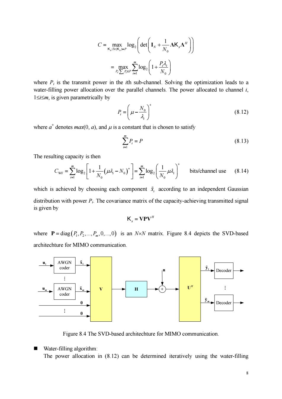
8 2 :( ) 0 1 max log det x x H N x Tr P C N I Λ Λ K K K 2 : 1 0 max log 1 i i i m i i P PP i P N where Pi is the transmit power in the ith sub-channel. Solving the optimization leads to a water-filling power allocation over the parallel channels. The power allocated to channel i, 1im, is given parametrically by 0 i i N P (8.12) where a+ denotes max(0, a), and is a constant that is chosen to satisfy 1 m i i P P (8.13) The resulting capacity is then WF 2 0 2 1 1 0 0 1 1 log 1 log m m i i i i C N N N bits/channel use (8.14) which is achieved by choosing each component i x according to an independent Gaussian distribution with power Pi. The covariance matrix of the capacity-achieving transmitted signal is given by H Kx VPV where 1 2 diag , ,., ,0,.,0 P PP Pm is an NN matrix. Figure 8.4 depicts the SVD-based architechture for MIMO communication. V + AWGN coder AWGN coder H Decoder Decoder H U um u1 1 x m x . . . 1 y m y n 0 0 Figure 8.4 The SVD-based architechture for MIMO communication. Water-filling algorithm: The power allocation in (8.12) can be determined iteratively using the water-filling
algorithm.We now describe it. We first set the iteration count p to1 and assume that所有(m-p+l)个并行子信道都使 .With this assumption,the constant is calculated(by substituting(8.12)into (8.13))as -》 Then we have n-pp空别 (8.15a) Using this value of the power allocated to the ith subchannel is given by -(-艾)-12m-pl (8.15b) If the power allocated to the channel with the lowest gain is negative(i.e.,P<). then we discard this channel by setting P=0 and return the algorithm with the iteration count p=p叶1.即迭代执行(8.15a)和(8.15b),将总功率P在剩余的(m-pr1)个子信道之间 进行分配。迭代计算直到获得的所有P≥0或一m为止。 8.3.3Ch nel Unknown to the Transmitter If the channel is known to the receiver,but not to the transmitter,then the transmitter cannot optimize its power allocation or input covariance structure across antennas.This implies that if the distribution of H follows the zero-mean spatially white(ZMSW)channel gain model,the signals transmitted from N antennas should be independent and the power should be equally divided among the transmit antennas,resulting an input covariance matrix Thus,the capacity in such a case is eaL.+sRmr)tw<N C={ bits per channel use (8.15) ea,+sNum小fw≥N where SNR=P/N.Using the SVD of H,we can express this as c-2e+-2+)
9 algorithm. We now describe it. We first set the iteration count p to 1 and assume that 所有(m-p+1)个并行子信道都使 用。With this assumption, the constant is calculated (by substituting (8.12) into (8.13)) as 1 0 1 m p i i N P Then we have 1 0 1 1 1 1 m p i i P N m p (8.15a) Using this value of , the power allocated to the ith subchannel is given by 0 , 1,2,., 1 i i N P i mp (8.15b) If the power allocated to the channel with the lowest gain is negative (i.e., 1 0 P m p ), then we discard this channel by setting 1 0 P m p and return the algorithm with the iteration count p = p+1. 即迭代执行(8.15a)和(8.15b),将总功率 P 在剩余的(m-p+1)个子信道之间 进行分配。迭代计算直到获得的所有 0 Pi 或 p=m 为止。 8.3.3 Channel Unknown to the Transmitter If the channel is known to the receiver, but not to the transmitter, then the transmitter cannot optimize its power allocation or input covariance structure across antennas. This implies that if the distribution of H follows the zero-mean spatially white (ZMSW) channel gain model, the signals transmitted from N antennas should be independent and the power should be equally divided among the transmit antennas, resulting an input covariance matrix x N P N K I . It is shown in [Telatar99] that this Kx indeed maximize the mutual information. Thus, the capacity in such a case is 2 2 log det , if log det , if H M H N M N N C M N N I HH I HH SNR SNR bits per channel use (8.15) where 0 SNR P N/ . Using the SVD of H, we can express this as 2 1 0 log 1 m ri i P C N 2 1 0 log 1 m i i P NN
-交e刘 bits/channel use (8.16) where Pn is the received signal power in the ith sub-channel.Equation (8.16)expresses the capacity of the MIMO channel as a sum of the capacities of m SISO channels,each having a power gain ofand transmit power P/N.(Note:Because of the use of complex signals,the above unit is sometimes expressed in terms of"bits/sec/Hz") Since the nonzero eigenvalues of HH"are the same as those of HH,the capacity of a channel with matrix H and H are the same.Furthermore,the capacity can be achieved by choosing independent1sism with each having independent Gaussian,zero-mean real and imaginary parts. 8.3.4 MIMO Capacity Examples Example I [Single antenna channel].Consider a channel with N=M=1 and H=h=1.The Shannon capacity of this channel is C=log:1+P =log2(1+y1h) bit/channel use (8.17) Example 2 [MIMO channel with coherent combining].Consider a MIMO channel withh=1 for all IsisN,IsjsM.We can write Has 「/M H=UDV#= (MN)[/N./N 1/M and we see that the diagonal matrix D will have only one nonzero entry M.Thus,the Shannon capacity of this channel is c-w别 (8.18) The x=V that achieves this capacity satisfies E[x]=P/N for all i.j.i.e.,the transmitters are all sending the same signal.Thus,we can see that H corresponds to such a system in which the same signal x is transmitted from N transmit antennas and the receiver performs coherent maximum ratio combining (MRC)by M antennas.Then (8.18)can be interpreted as follows The received signal at antenna i is given by y=Nx and the received signal power at P antenna i is P.=N2 Since each receiver sees the same signal,and the noises at the
10 2 1 log 1 m i i N SNR bits/channel use (8.16) where Pri is the received signal power in the ith sub-channel. Equation (8.16) expresses the capacity of the MIMO channel as a sum of the capacities of m SISO channels, each having a power gain of i and transmit power P/N. (Note: Because of the use of complex signals, the above unit is sometimes expressed in terms of “bits/sec/Hz”.) Since the nonzero eigenvalues of HHH are the same as those of HHH, the capacity of a channel with matrix H and HH are the same. Furthermore, the capacity can be achieved by choosing independent { ,1 } i x i m with each i x having independent Gaussian, zero-mean real and imaginary parts. 8.3.4 MIMO Capacity Examples Example 1 [Single antenna channel]. Consider a channel with N=M=1 and H=h=1. The Shannon capacity of this channel is 2 2 2 2 0 | | log 1 log 1 | | P h C h N bit/channel use (8.17) Example 2 [MIMO channel with coherent combining]. Consider a MIMO channel with hij=1 for all 1iN, 1jM. We can write H as 1/ 1/ 1/ 1/ H M MNN N M H UDV and we see that the diagonal matrix D will have only one nonzero entry MN . Thus, the Shannon capacity of this channel is 2 0 log 1 P C MN N (8.18) The x Vx that achieves this capacity satisfies * [] / E i j xx P N for all i, j; i.e., the transmitters are all sending the same signal. Thus, we can see that H corresponds to such a system in which the same signal x is transmitted from N transmit antennas and the receiver performs coherent maximum ratio combining (MRC) by M antennas. Then (8.18) can be interpreted as follows. The received signal at antenna i is given by i y Nx and the received signal power at antenna i is 2 ri P P N N . Since each receiver sees the same signal, and the noises at the