xEA,by the group property,then A+x=A.This implies that a lattice is"geometrically uniform,”every nt of the lattice has the same number of neighbors at each distance. and all decision regions of a minimum distance decode ("Voronoi regions")are congruent and form a tessellation ofR" Asublattice A'ofa given lattice A is a subset of the points in A that is itself a lattice.The lcostsof a sublattice is denoted by and is called a partition ofnot A=AO[A/AT=AU(A'+x) (5.2) where x is chosen such that (A'+x)A.(There are g cosets in a q-ary partition.)For example,2=RZ2+(0,0).(0,1)) ·。·。· 。 。 。 。年华年。海年 。&。0 ●年。●。 ●0●。0◆0 222 Fig 5.10 llustration of the binary partition chainR The nearest neighbor quantizer (is defined by e(y)=xEA,if lly-xlslly-x'll,Vx'EA The fiundamental Voronoi region of A is the set of points in R"closest to the zero codeword;i.e., 名={y∈R"I2y)=0 The Voronoi region associated with x is the set of points y such that (y)x,and is given by a shift of by x.Note that other fundamental regions exist. ●A fundamental parallelotope of the lattice is the paralleltope(超平行体)that consists of the points{aGla∈[0,lyr} A fundamental parallelotope is an example of a fundamental region for the lattice;i.e.,a building block which when repeated many times fills the whole space with just one lattice 5-10
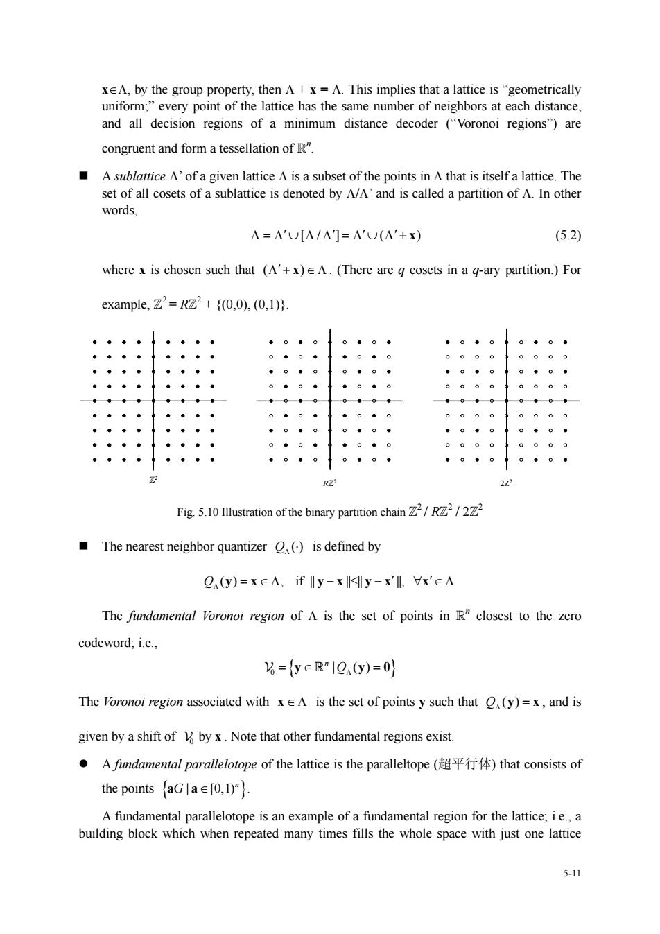
5-11 x∈Λ, by the group property, then Λ + x = Λ. This implies that a lattice is “geometrically uniform;” every point of the lattice has the same number of neighbors at each distance, and all decision regions of a minimum distance decoder (“Voronoi regions”) are congruent and form a tessellation of Rn . A sublattice Λ’ of a given lattice Λ is a subset of the points in Λ that is itself a lattice. The set of all cosets of a sublattice is denoted by Λ/Λ’ and is called a partition of Λ. In other words, Λ=Λ ∪ Λ Λ =Λ ∪ Λ + ′ [/ ] ( ) ′′′ x (5.2) where x is chosen such that ( ) Λ + ∈Λ ′ x . (There are q cosets in a q-ary partition.) For example, Z2 = RZ2 + {(0,0), (0,1)}. Z2 RZ2 2Z2 Fig. 5.10 Illustration of the binary partition chain Z2 / RZ2 / 2Z2 The nearest neighbor quantizer ( ) QΛ ⋅ is defined by Q ( ) , if || || || ||, Λ y x yx yx x = ∈Λ − ≤ − ∀ ∈Λ ′ ′ The fundamental Voronoi region of Λ is the set of points in Rn closest to the zero codeword; i.e., 0 { | () } n = ∈ = QΛ V y y R 0 The Voronoi region associated with x ∈Λ is the set of points y such that ( ) QΛ y = x , and is given by a shift of 0 V by x . Note that other fundamental regions exist. z A fundamental parallelotope of the lattice is the paralleltope (超平行体) that consists of the points { | [0,1) }n a a G ∈ . A fundamental parallelotope is an example of a fundamental region for the lattice; i.e., a building block which when repeated many times fills the whole space with just one lattice
point in each copy.Fig.5.11 shows that around each lattice point is a region known as the undamental parallelotope(用阴影表示) Fig.5.11 The fundamental parallelotopes around the lattice points. The key geometrical parameters of a lattice A are (a)the minimum squared Euclidean distance d2(A)between lattice points; (b)the kissing number K(A),which is the number of nearest neighbors to any lattice point. (c)the fundamental volume V(A),which is the volume of the n-space corresponding to each lattice point.As indicated in Fig.5.11,this volume is the volume of the fundamental region.Let A=GG".It can be shown that V(A)det()2=det(G)for any generator matrix GofA These parameters will directly affect the performance of a lattice constellation(lattice code) A normalized density parameter d(A) will be identified as the nomial coding gain Definition 2:A lattice constellation C(A,R)=(A+t)oR is the finite set of points in a lattice translate A+t that lie within a compact bounding regionR of n-space. (Note:A lattice is constrained to have a point at zero.The translate vector t make the resulting constellation has no point at zero.The intersection of A with the regionR results in a finite 5-12
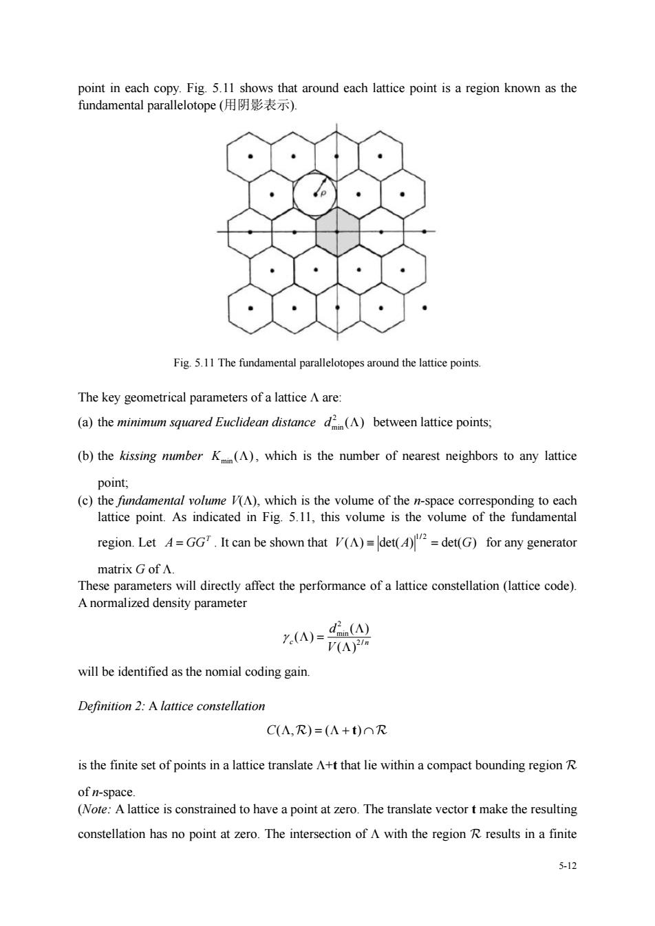
5-12 point in each copy. Fig. 5.11 shows that around each lattice point is a region known as the fundamental parallelotope (用阴影表示). Fig. 5.11 The fundamental parallelotopes around the lattice points. The key geometrical parameters of a lattice Λ are: (a) the minimum squared Euclidean distance 2 min d ( ) Λ between lattice points; (b) the kissing number min K ( ) Λ , which is the number of nearest neighbors to any lattice point; (c) the fundamental volume V(Λ), which is the volume of the n-space corresponding to each lattice point. As indicated in Fig. 5.11, this volume is the volume of the fundamental region. Let T A GG = . It can be shown that 1/2 V AG ( ) det( ) det( ) Λ≡ = for any generator matrix G of Λ. These parameters will directly affect the performance of a lattice constellation (lattice code). A normalized density parameter 2 min 2 / ( ) ( ) ( ) c n d V γ Λ Λ = Λ will be identified as the nomial coding gain. Definition 2: A lattice constellation C(, ) ( ) Λ R R = Λ+ ∩t is the finite set of points in a lattice translate Λ+t that lie within a compact bounding region R of n-space. (Note: A lattice is constrained to have a point at zero. The translate vector t make the resulting constellation has no point at zero. The intersection of Λ with the region R results in a finite

number of points in the constellation.) Example 5.3.2:An M-PAM constellation 3.(M-1))is a one-dimensional lattice constellation C(2Z,R)with A+t=2Z+1 and R=[-M.Ml. Some 2D lattice constellations are shown in Fig.12. Fig.12 Two-dimensional constellations based on the integer lattice The key geometric properties of the region R are (a)its volume V(R)=[dx; (b)the average energy P(R)per dimension of a uniform probability density function overR A-1念 (5.3) For performance analysis of large lattice constellations,we use the following approximations Fomey call this the contimous approximation). The continuous approximation: (a)The size of the constellation C(A,R)(i.e.,the number of signal points in C(A,R))is well approximated by V(R)/V(A). (b)When the number of points in C(A,R)is large,a uniform discrete distribution of the points over C(A,R)is well approximated by a uniform continuous distribution over 5-13
5-13 number of points in the constellation.) Example 5.3.2: An M-PAM constellation {±1, ±3,., ±(M-1)} is a one-dimensional lattice constellation C(2Z, R) with Λ+t =2Z+1 and R=[-M, M]. Some 2D lattice constellations are shown in Fig. 12. 16-QAM 64-QAM 32-QAM 256-QAM 128-QAM Fig.12 Two-dimensional constellations based on the integer lattice Z2 . The key geometric properties of the region R are (a) its volume ( ) V d = ∫ x R R ; (b) the average energy P(R) per dimension of a uniform probability density function over R: 2 || || ( ) ( ) d P n V = ∫ x x R R R (5.3) For performance analysis of large lattice constellations, we use the following approximations (Forney call this the continuous approximation). The continuous approximation: (a) The size of the constellation C(Λ, R) (i.e., the number of signal points in C(Λ, R)) is well approximated by ( ) / ( ) V V R Λ . (b) When the number of points in C(Λ, R) is large, a uniform discrete distribution of the points over C(Λ, R) is well approximated by a uniform continuous distribution over
the region R.Thus.the average energy per dimension of a signal constellation is P(C(A,R)》≈P(R) (c)The average number of nearest neighbors to any point in C(A,R)isK(A). Example 5.3.3:For R=-M.M],the parameters are V(R)=2M,P(R)=M/3 When n=2,and the shaping gain is an 2rx2r square,we have VR)=(2r),and V(R)=2.If X=(X1,X2)is uniformly distributed over the circle,then P(R)=E[llX]P1/2 5.3.I Shaping and Coding Gain Under the continuous approximation,the coding gain for a lattice code is separable into hen),which depends on the reaive spacing of points in. but is independent of 2)The shaping gain(R).which is determined by the choice of the signal constellation bounding regionR Consider the probability of decoding error for a lattice constellation A used over an AWGN channel.The union bound estimate(UBE)is P(e)K(A) d2() V 4 where is the noise power per dimension. Sirce)c where 4G2 4P(C(A,R)2(2”-) 4P(C(,R) is a parameter of the constellation,the UBE can be written as P(e)≈K=()(VP.SNR】 Using the continuous approximation,we have 5-14
5-14 the region R. Thus, the average energy per dimension of a signal constellation is PC P ( ( , )) ( ) Λ R R ≈ (c) The average number of nearest neighbors to any point in C(Λ, R) is ≈ min K ( ) Λ . Example 5.3.3: For R=[-M, M], the parameters are V(R) = 2M, P(R) = M2 /3. When n=2, and the shaping gain is an 2r×2r square, we have V(R)=(2r) 2 , and 2 2 2 2 1 2 12 1 1 ( ) 24 3 r r r r r x x dx dx r − − =× + = ∫ ∫ . When the shaping region R is a circle with radius r, V(R) =πr 2 . If X=(X1, X2) is uniformly distributed over the circle, then P(R) = E[||X||2 ]/2 = 2 1 E X[ ], where 2 21 2 21 2 2 2 1 1 21 2 1 [ ] 4 r rx r rx r E X x dx dx πr − − −− = = ∫ ∫ . 5.3.1 Shaping and Coding Gain Under the continuous approximation, the coding gain for a lattice code is separable into two parts: 1) The fundamental coding gain γc(Λ), which depends on the relative spacing of points in Λ, but is independent of R. 2) The shaping gain γs(R), which is determined by the choice of the signal constellation bounding region R. Consider the probability of decoding error for a lattice constellation Λ used over an AWGN channel. The union bound estimate (UBE) is 2 min min 2 ( ) () ( ) 4 d Pe K Q σ ⎛ ⎞ Λ ≈ Λ ⎜ ⎟ ⎝ ⎠ where σ 2 is the noise power per dimension. Since 2 2 min min 2 2 norm ( ) ( )(2 1) ( ( , )) 4 4 ( ( , )) (2 1) d d PC SNR P C ρ ρ γ σ σ Λ Λ− Λ = ⋅ =⋅ Λ − R R , where 2 min ( )(2 1) 4 ( ( , )) d P C ρ γ Λ − = Λ R is a parameter of the constellation, the UBE can be written as P e K Q SNR () ( ) ≈Λ ⋅ min norm ( γ ) Using the continuous approximation, we have

p-2a网28 SWR=PCAR》P.PE σ2(2P-1)V(R)2Nσ (R) (A VA y 4P(R) =3y.(A)Y(R) where (5.4) is defined as the nominal (or asymptotic)coding gain of A,and (R)=R 12P(R) (5.5) is defined as the shaping gain ofR The nominal coding gain (A)measures the increase in density of A over the baseline integer lattice Z".The shaping gain(R)measures the decrease in average energy ofR relative to an n-cube [-b.b]".It can be shown that, given any lattice constellation C.the nominal coding and shaping gains of any K-fold Cartesian product constellation C is the same as those of C Example 5.3.4:For the square constellation,n=2,shaping regionR is a 2rx2r square.Then (R)=,(R) 1.Since V(A)(A),we have A)=1.and so3 From the discussion above,the probability of block decoding error per two dimensions is (e)=K,(A)((A),(R)-3SNR.) (5.6 where K(A)=2K(A)/n is the normalized error coefficient per two dimensions. Note that the nominal coding gain is based solely on the argument of the (.)function in the UBE,which bec omes inf r dens onal latti ces s.On the other hand, as before,the effective coding gain is limited by the number of nearest neighbors. error coefficient Kmin(A).which becomes very large for high-dimensional dense lattices.In fact,the Shannon limit shows that no lattice can have a combined effective coding gain and shaping gain greater than 9dB at P(e)=10e-6.This limits the maximum possible effective 15
5-15 2 2 2 2 () log | ( , ) | log ( ) V C n nV ρ = Λ≈ Λ R R 2 / norm 2 2/ 2 ( ( , )) ( ) ( ) (2 1) ( ) n n PC V P SNR V ρ σ σ Λ Λ = ≈⋅ − R R R 2 / 2 min ( ) ( ) ( ) 3()( ) 4( ) n c s V d V P γ γγ ⎛ ⎞ Λ ⎜ ⎟ ⎝ ⎠ Λ ≈ =Λ R R R where 2 min 2 / ( ) ( ) ( ) c n d V γ Λ Λ = Λ (5.4) is defined as the nominal (or asymptotic) coding gain of Λ, and 2 / ( ) ( ) 12 ( ) n s V P γ = R R R (5.5) is defined as the shaping gain of R. The nominal coding gain γc(Λ) measures the increase in density of Λ over the baseline integer lattice Zn . The shaping gain γs(R) measures the decrease in average energy of R relative to an n-cube [-b, b] n . It can be shown that, given any lattice constellation C, the nominal coding and shaping gains of any K-fold Cartesian product constellation CK is the same as those of C. Example 5.3.4: For the square constellation, n=2, shaping region R is a 2r×2r square. Then 2 2 () 4 () 1 12 ( ) 12 / 3 s V r P r γ == = × R R R . Since 2 min V d () () Λ = Λ , we have γc(Λ)=1, and so γ=3. From the discussion above, the probability of block decoding error per two dimensions is P e K Q SNR s s cs () ( ) ( ) ( )3 ≈Λ Λ ⋅ ( γ γ R norm ) (5.6) where min ( ) 2 ( )/ K Kn s Λ= Λ is the normalized error coefficient per two dimensions. Note that the nominal coding gain is based solely on the argument of the Q(.) function in the UBE, which becomes infinite for dense n-dimensional lattices as n→∞. On the other hand, as before, the effective coding gain is limited by the number of nearest neighbors; i.e., the error coefficient Kmin(Λ), which becomes very large for high-dimensional dense lattices. In fact, the Shannon limit shows that no lattice can have a combined effective coding gain and shaping gain greater than 9dB at P(e)=10e-6. This limits the maximum possible effective