同济大学：《结构动力学》课程教学资源（教案讲义）Lecture 06 Numerical Evaluation of Dynamic Response

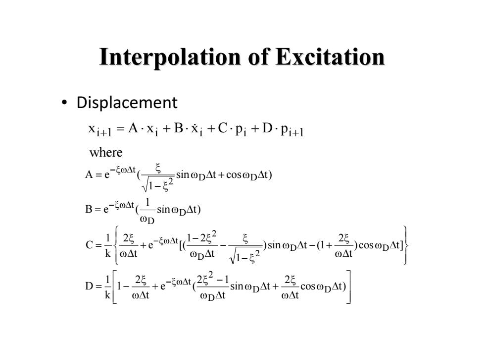
Interpolation of Excitation 。Displacement Xi+1=A.Xi+B.xi+C.Pi+D.Pi+l where A=e-ioAt(E 5 sin@D△t+cos@pAt) V1-2 B=e(sin@DAt) OD 1 C- )sinopat-()cosopat) ko△t ODAt 1-g2 D= 1- k o△t OD△t O△t

Interpolation of Excitation Interpolation of Excitation • Displacement i 1 i i i i 1 x A x B x C p D p            where )tcostsin 1 (eA DD 2 t           )tsin 1 (eB D D t                                   ]tcos) t 2 1(tsin) 1 t 21 [(e t 2 k 1 C DD 2 D 2 t                          )tcos t 2 tsin t 12 (e t 2 1 k 1 D DD D 2 t

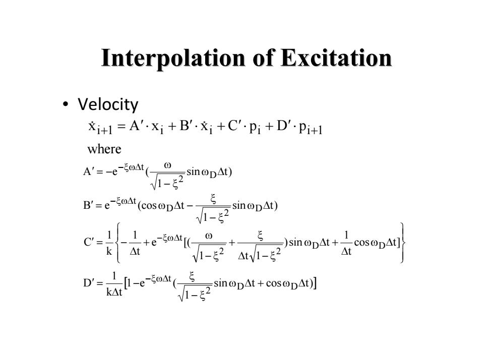
Interpolation of Excitation ·Velocity i+=A'.xi+B'.xi+C'Pi+D'.Pi+l where A'=-e-ioAt- sin@pAt) V1-2 B'-e-At(cosDAt- -sinoDAt) V1-2△W1-2

Interpolation of Excitation Interpolation of Excitation • Velocity xi1 A xi B xi C pi D pi1           where )tsin 1 (eA D 2 t          )tsin 1 t(coseB D 2 D t                                        ]tcos t 1 tsin) 1t1 [(e t 1 k 1 C DD 22 t  )tcostsin  1 (e1 tk 1 D DD 2 t             

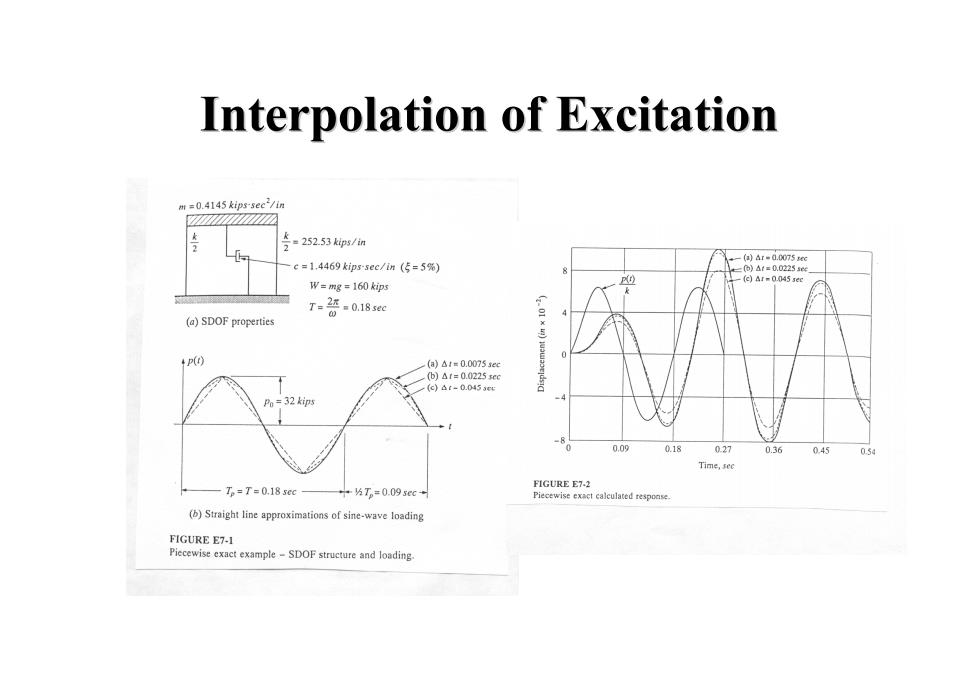
Interpolation of Excitation m=0.4145 kips-sec?/in =252.53ks/n +-()ar=0.0075 =1.4469 kips-sec/im(5=5%) (c)Ar=0.045se W=mg =160 kips 7语018 (a)SDOF properties (a)△1m0.00755eg b△1=0.0225eg (c）dt-0.0453e Po=32 kips 0.09 018 027 0.36 045 058 Time,sec —T。=T=0.18s0c FIGURE E7.2 中5T=0.09scc Piecewise exact calculated response (b)Straight line approximations of sine-wave loading FIGURE E7-1 PiecewiseexacxmpeSDOFstrureand loading

Interpolation of Excitation Interpolation of Excitation

Interpolation of Excitation 。Note: -Feasible only for linear system -SDOF system:impractical for MDOF -Accuracy depends on the linear interpolation of loading p

Interpolation of Excitation Interpolation of Excitation • Note: –Feasible only for linear system – SDOF system: impractical for MDOF – Accuracy depends on the linear interpolation of loading p

Time-Domain Analysis .(1)Interpolation of Excitation Method .(2)Central Difference Method ·(3)Newmark's Method ·(4)Wilson-θMethod (5)State space method

Time-Domain Analysis • (1) Interpolation of Excitation Method • (2) Central Difference Method • (3) Newmark’s Method • (4) Wilson- Method • (5) State space method 