[1110100 H=0111010 (4.2) [0011101 X X X Figure 6.10 Normal graph for parity-check realization of (3)Hamming code Fig.4.6.11 shows a normal graph of a turbo code. info bits first second parity parity bits 百 bits 百 百 trellis 1 trellis 2 Fig 4.6.11 Normal graph ofa classical turbo code A More General Description from a Factorization Perspective Normal graph is also called the Forney-style factor graph(FFG).The term"factor graph" results from the fact that an FFG is a diagram that represents the factorization of a function of several variables.Assume,for example,that some functionf(u.x.y.=)can be factored as f(,w,x,八,)=fu,w,x)(x,)(e) (4.3) This factorization is expressed by the FFG shown in Fig.4.6.12.The factors are also called local functions,and their product is called the global function.In (4.3),the global function isf andi,are the local functions.In general,an FFG is defined by the following rules: 11
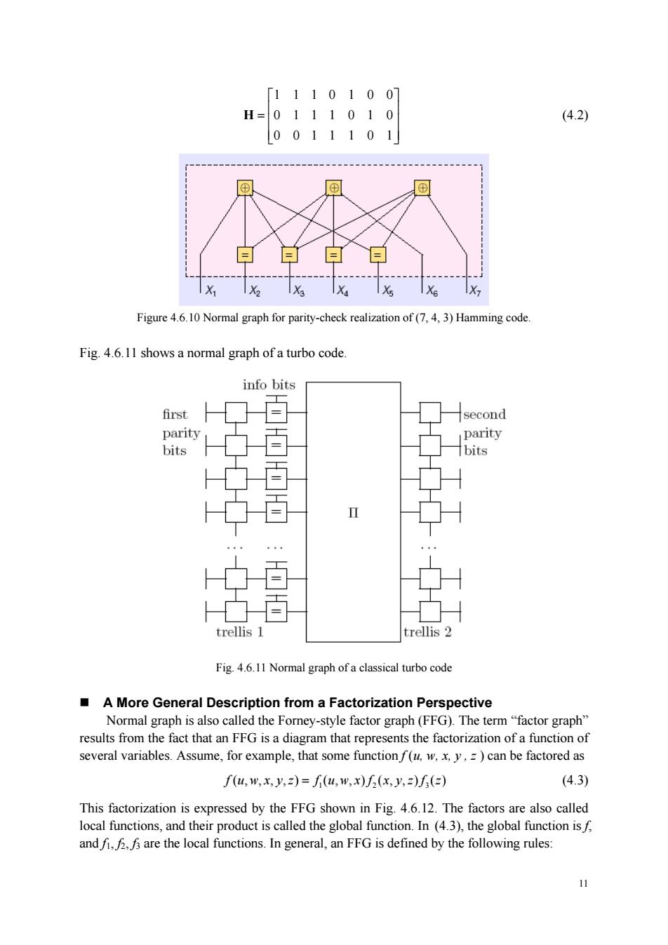
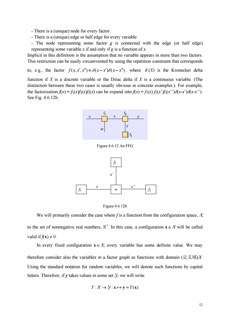
11 1110100 0111010 0011101 ⎡ ⎤ ⎢ ⎥ = ⎣ ⎦ H (4.2) Figure 4.6.10 Normal graph for parity-check realization of (7, 4, 3) Hamming code. Fig. 4.6.11 shows a normal graph of a turbo code. Fig. 4.6.11 Normal graph of a classical turbo code A More General Description from a Factorization Perspective Normal graph is also called the Forney-style factor graph (FFG). The term “factor graph” results from the fact that an FFG is a diagram that represents the factorization of a function of several variables. Assume, for example, that some function f (u, w, x, y , z ) can be factored as 1 23 f (, , ,) (, , ) (, ,) () uwxyz f uwx f xyz f z = (4.3) This factorization is expressed by the FFG shown in Fig. 4.6.12. The factors are also called local functions, and their product is called the global function. In (4.3), the global function is f, and f1, f2, f3 are the local functions. In general, an FFG is defined by the following rules:
There is a (unique)node for every factor. representing some variable x if and only if g is a function ofx. Implicit in this definition is the assumption that no variable appears in more than two factors. This restriction can be easily circumvented by using the repetition constraint that corresponds to.e.g.the factor f(x.x'x")=6(x-x)(x-x"),where (X)is the Kronecker delta function if is a discrete variable or the Dirac delta if is a continuous variable.(The distinction between these two cases is usually obvious in concrete examples.).For example, the factorization fx)=fi(xx(x)can be expand into fx)=fi(x)(x(x)x-x)x-x"). See Fig.4.6.12b. Figure4.6.12 An FFG E Figure4.6.12b We will primarily consider the case where fis a function from the configuration space, to the set of nonnegative real numbers,R".In this case,a configuration xe&will be called valid iff)≠0. In every fixed configuration xe every variable has some definite value.We may therefore consider also the variables in a factor graph as functions with domain(定义域),X Using the standard notation for random variables,we will denote such functions by capital letters.Therefore,ify takes values in some set,we will write Y:X→y:x→y=Y(x)
12 - There is a (unique) node for every factor. - There is a (unique) edge or half edge for every variable. - The node representing some factor g is connected with the edge (or half edge) representing some variable x if and only if g is a function of x. Implicit in this definition is the assumption that no variable appears in more than two factors. This restriction can be easily circumvented by using the repetition constraint that corresponds to, e.g., the factor f (, , ) ( )( ) xx x x x x x ′ ′′ ′ ′′ ≡− − δ δ , where δ(X) is the Kronecker delta function if X is a discrete variable or the Dirac delta if X is a continuous variable. (The distinction between these two cases is usually obvious in concrete examples.). For example, the factorization f(x) = f1(x)f2(x)f3(x) can be expand into f(x) = f1(x) f2(x’)f3(x’’)δ(x-x’)δ(x-x’’). See Fig. 4.6.12b. Figure 4.6.12 An FFG Figure 4.6.12b We will primarily consider the case where f is a function from the configuration space, X, to the set of nonnegative real numbers, R+ . In this case, a configuration x∈X will be called valid if f(x) ≠ 0. In every fixed configuration x∈X, every variable has some definite value. We may therefore consider also the variables in a factor graph as functions with domain (定义域)X. Using the standard notation for random variables, we will denote such functions by capital letters. Therefore, if y takes values in some set Y, we will write Y Y : : () X Y → = x 6 y x = x x’’ x’ f1 f2 f3