(i().(sj(k)=()of local variable values.The set of all local configurations is a vector space -(Lx几 A linear local constraint code is a subspace C whose codewords are precisely the valid local configurations which may actually occur. The full behaviorBS generated by the realization is the set of all combinations(x,s) (called trajectories)of symbol and state configurations that satisfy all local constraints 2B={L,s)eX×SI(zv)eC,k∈K The code Cgenerated by the realization is the set of all symbol sequencesx that appear in any trajectory(亿,s)eB.In other words,C=Be Notice that the constraint imposed by a linear homogeneous equation that involvesr=n-k variables is equivalent to a constraint that these variables must lie in a certain (r-1)-dimensional subspace of F;i.e.,that they form a codeword in a(r,-)linear block code over F Example:Consider a conventional state-space realization of Con the time axis I=[0,n). A trellis diagram is a detailed graphical model of a conventional state-space realization We define state dimension for the state time =0;i.e.,the starting and ending state space have size So==1.We then define each trellis section by a linear subspace (called branch space)CFi,which defines the set of state transitions (s)xthat can possibly occur and the code symbol x,Fassociated with each such transition.In other words,the behavioral constraint at time i is that the tripe (s)must lie in a certain small linear block code Cof lengthn ++1 over F Thus,each state variable S,is involved in two constraints,C and C while each symbol variableX is involved in the single constraint C.Each valid local configuration
6 {( ) ( )} ( ) |() | () , (), , () , i j kk xi k s j k ∈ ∈= x s I J I J of local variable values. The set of all local configurations is a vector space () () ki j ik j k ∈ ∈ ⎛ ⎞⎛ ⎞ = × ⎜ ⎟⎜ ⎟ ⎝ ⎠⎝ ⎠ ∏ ∏ I J VX S A linear local constraint code is a subspace Ck ⊆Vk whose codewords are precisely the valid local configurations which may actually occur. The full behavior B⊆X ×S generated by the realization is the set of all combinations (x, s) (called trajectories) of symbol and state configurations that satisfy all local constraints B = ∈× ∈ ∈ {( , ) | ( , ) , xs x s XS C K | () | () I J kk k k } The code C generated by the realization is the set of all symbol sequences x that appear in any trajectory (x, s)∈B. In other words, C = B|X. Notice that the constraint imposed by a linear homogeneous equation that involves r =n-k variables is equivalent to a constraint that these variables must lie in a certain (r-1)-dimensional subspace of r F q ; i.e., that they form a codeword in a (r, r-1) linear block code over Fq. Example: Consider a conventional state-space realization of C on the time axis I = [0, n). A trellis diagram is a detailed graphical model of a conventional state-space realization. We define state space j j q μ S = F of dimension μj for the state time axis J=[0, n], where μ0 = μn = 0; i.e., the starting and ending state space have size |S0|=|Sn|=1. We then define each trellis section by a linear subspace (called branch space) Ci ⊆Si×Si+1×Fq, i∈I, which defines the set of state transitions 1 1 (, ) ii i i s s + + ∈ × S S that can possibly occur and the code symbol xi∈Xi=Fq associated with each such transition. In other words, the behavioral constraint at time i is that the tripe (si, si+1, xi) must lie in a certain small linear block code Ci of length ni=μi +μi+1 +1 over Fq. Thus, each state variable Si is involved in two constraints, Ci and Ci-1, while each symbol variable Xi is involved in the single constraint Ci-1. Each valid local configuration
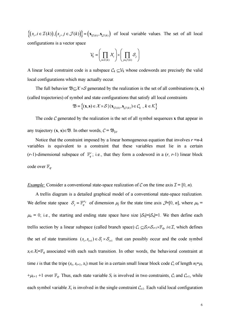
(s,x)EC is a set of variables that satisfy the constraints at time i and corresponds to a distinct valid trellis branch labeled by the corresponding(s),so the branch complexity at time i is the size Cof the local constraint code C. The full behavior of this realization is then the set of all state/symbol sequences(s,x) such that ()C,1sisn,which is a set of linear homogeneous constraints.For each valid configuration (s,x)in the state sequence s represents a valid path through the code trellis.and the symbol sequence x represents the corresponding codeword.The code generated by the trellis diagram is the set of all path label sequences,namely,the projection C-Bur As an example,Fig.4.6.3 shows the trellis diagram for the(8,4,4)RM code.It is known that,for the(84,4)code,the minimal state complexity profile of any trellis diagram is given by (o)=(1.2.4.8.4.8.4.2,1).The state spaces at time =1.2. may be defined by their F2 components as follows:s=(s),5=(s21,2),(,3). 0 0 0 Figure 4.6.3 The trellis diagram for the(8,4,4)code The main difficulty with trellises and other cycle-free graph representations of codes is as codes become more powerf the alphabets (state space)of the state variab necessarily bec which ever makes trellis-type decoding algorithms impractical. 4.6.5 Graphs of General Linear Behavioral Representations-Factor Graph tare various styles for drawing graphs of general linear behavioral representations. We start with ralized Tanner ow called factor graphs).A fact graph is a Tanner grah that may contain auxiliary (state)variables.In a factor aph.two types of vertices represent variable m-tuples and constraint codes,respectively.Again,an edge connects a variable vertex to a constraint vertex if and only if the corresponding variable is involved in the corresponding constraint code
7 1 (, , ) ii i i ss x + ∈C is a set of variables that satisfy the constraints at time i and corresponds to a distinct valid trellis branch labeled by the corresponding (si, si+1, xi), so the branch complexity at time i is the size |Ci| of the local constraint code Ci. The full behavior B of this realization is then the set of all state/symbol sequences (s, x) such that (si, si+1, xi) ∈ Ci, 1≤i≤n, which is a set of linear homogeneous constraints. For each valid configuration (s, x) in B, the state sequence s represents a valid path through the code trellis, and the symbol sequence x represents the corresponding codeword. The code generated by the trellis diagram is the set of all path label sequences, namely, the projection C=B|X. As an example, Fig. 4.6.3 shows the trellis diagram for the (8, 4, 4) RM code. It is known that, for the (8,4,4) code, the minimal state complexity profile of any trellis diagram is given by (|S0|,|S1|,|S2|,|S3|,|S4|,|S5|,|S6|,|S7|,|S8|) = (1,2,4,8,4,8,4,2,1). The state spaces at time i=1,2,. may be defined by their F2 components as follows: s1=(s11), s2=(s21, s22), s3=(s31, s32, s33),. Figure 4.6.3 The trellis diagram for the (8, 4, 4) code. The main difficulty with trellises and other cycle-free graph representations of codes is that as codes become more powerful, the alphabets (state space) of the state variables must necessarily become exponentially large, which eventually makes trellis-type decoding algorithms impractical. 4.6.5 Graphs of General Linear Behavioral Representations – Factor Graph There are various styles for drawing graphs of general linear behavioral representations. We start with generalized Tanner graphs (now called factor graphs). A factor graph is a Tanner graph that may contain auxiliary (state) variables. In a factor graph, two types of vertices represent variable m-tuples and constraint codes, respectively. Again, an edge connects a variable vertex to a constraint vertex if and only if the corresponding variable is involved in the corresponding constraint code
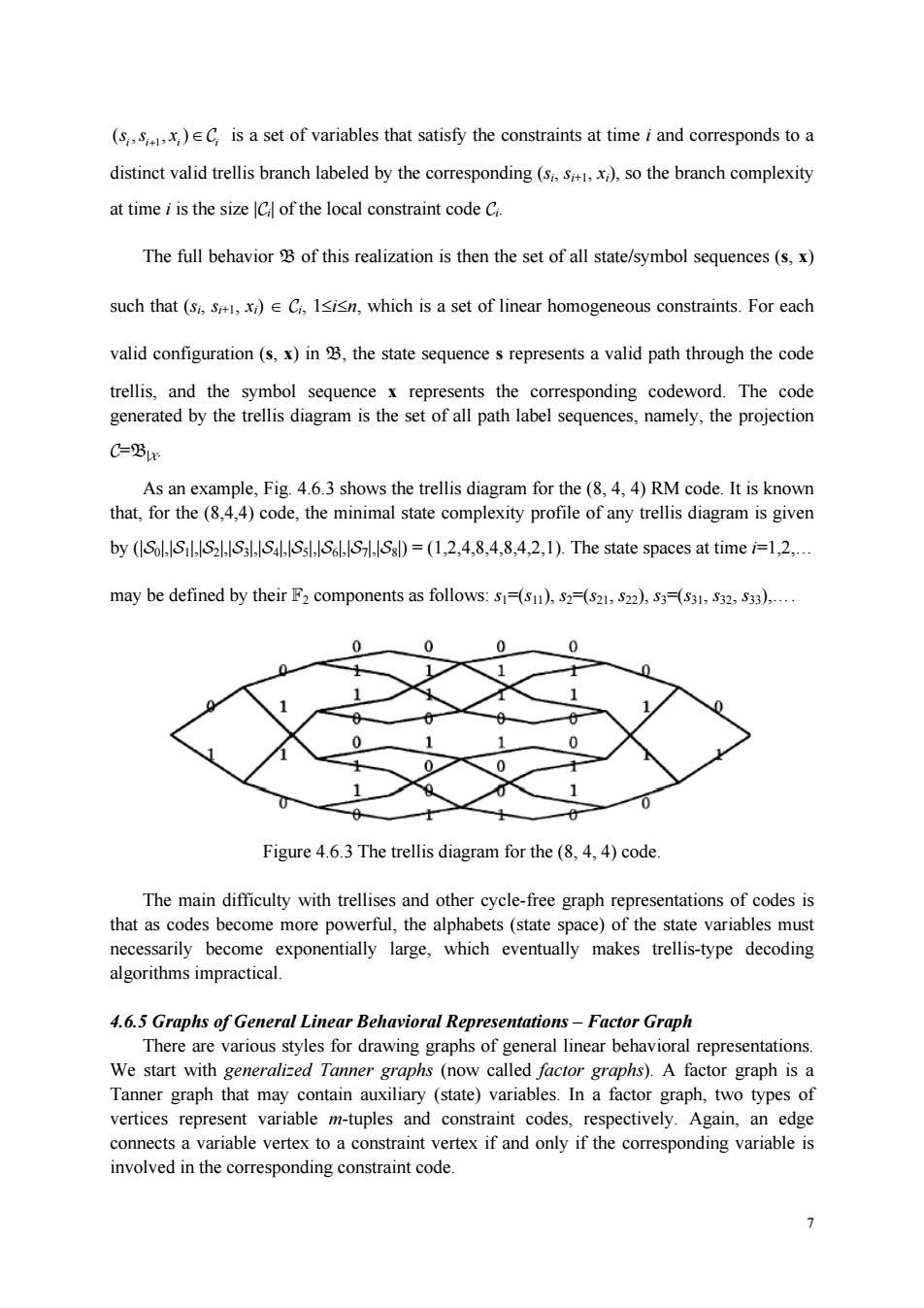
A generic factor graph is shown in Fig.4.6.4,where symbol m-tuples are represented by filled circles, ○ Figure 4.6.4 A factor graph Fig.4.6.5 is a factor graph of the trellis realization of (84,4)code.Each state variable is labeled by the dimension of its alphabet.Each constraint code C is labeled by its length and dimension (n,k),where n=+.+1 and k=log,C Since the symbol variables have degree 1,we use the special"dongle"symbol for them. 囟-③白-③应③区-③-应@囟-⑧应-③□ (2,1)1(4,2)2(6,3)3(G,3)26,3)3(6,3)2(4,2)1(2,1) Figure 4.6.5 Factor graph for the trellis realization of (8,4,4)code 4.6.6 The Forney-Style Factor Graphs-Normal Graphs Normal were proposed by Forney in 1998,in which co straint codes are represented by vertices,but variables are represented by edges(if the variable has degree 2)o by hyper edges(if the variable has degree other than 2). Normal graphs are particularly nice when the realizations are normal realizations.We define a realization to be normal if the degree of every symbol variable is 1,and the degree of every state variable W then represent symbol variables as before by hal-edgesn the ”symbols,.and by ordinary edges.Fig.6.6 shows an rcsnttion of ()de Ii seen that nommal r may be simpler
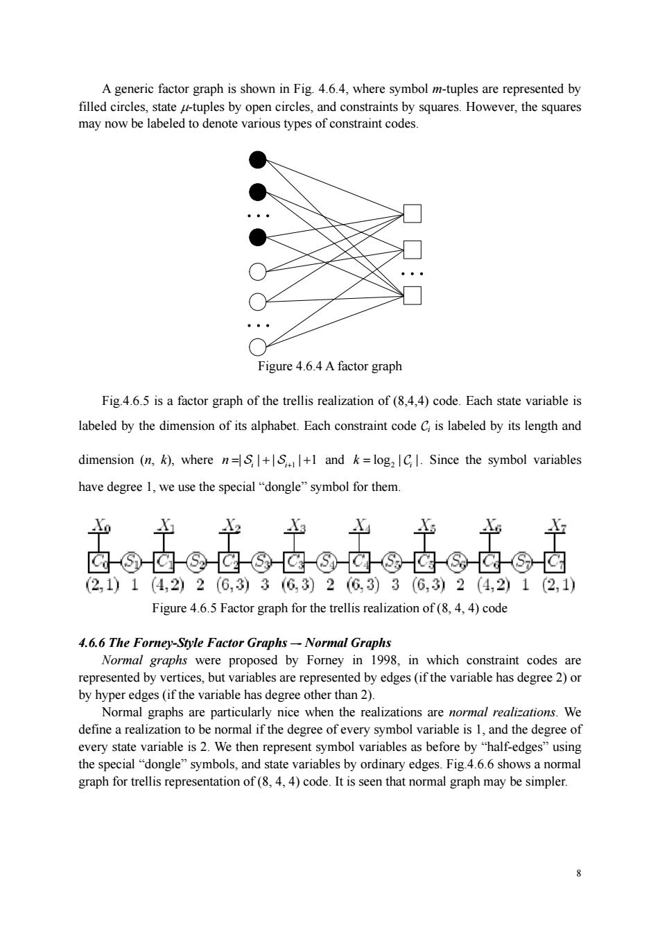
8 A generic factor graph is shown in Fig. 4.6.4, where symbol m-tuples are represented by filled circles, state μ-tuples by open circles, and constraints by squares. However, the squares may now be labeled to denote various types of constraint codes. Figure 4.6.4 A factor graph Fig.4.6.5 is a factor graph of the trellis realization of (8,4,4) code. Each state variable is labeled by the dimension of its alphabet. Each constraint code Ci is labeled by its length and dimension (n, k), where 1 | | | |1 i i n =+ + S S + and 2 log | | i k = C . Since the symbol variables have degree 1, we use the special “dongle” symbol for them. Figure 4.6.5 Factor graph for the trellis realization of (8, 4, 4) code 4.6.6 The Forney-Style Factor Graphs –- Normal Graphs Normal graphs were proposed by Forney in 1998, in which constraint codes are represented by vertices, but variables are represented by edges (if the variable has degree 2) or by hyper edges (if the variable has degree other than 2). Normal graphs are particularly nice when the realizations are normal realizations. We define a realization to be normal if the degree of every symbol variable is 1, and the degree of every state variable is 2. We then represent symbol variables as before by “half-edges” using the special “dongle” symbols, and state variables by ordinary edges. Fig.4.6.6 shows a normal graph for trellis representation of (8, 4, 4) code. It is seen that normal graph may be simpler. . .

3 7 2,1) 4.2) 63) 6,3) (6,3) 4.2 2.1) Figure 4.6.6 Normal graph for trellis representation of(8,4,4)code Any realization may be transformed inta normal realization by simpe in Fi4.7.The conversion from a factor grap toa norma replications and state replications,as shown in Fig.4.6.8.In the normal graph,all graph vertices represent constraints,and the repetition constraints (or,equality constraints)are represented by vertices labeled by the symbol"=". = Figure 4.6.7 Normal graph with observed variables (represented by "dongles"),equality constraints and zero-sum constraints(represented by squares with"+"). Figure 4.6.8 As an example,Fig.4.6.9 shows the normal graph of the(8,4,4)code defined in (4.1)
9 Figure 4.6.6 Normal graph for trellis representation of (8, 4, 4) code Any realization may be transformed into a normal realization by simple conversion shown in Fig. 4.6.7. The conversion from a factor graph to a normal graph involves symbol replications and state replications, as shown in Fig. 4.6.8. In the normal graph, all graph vertices represent constraints, and the repetition constraints (or, equality constraints) are represented by vertices labeled by the symbol “=”. Figure 4.6.7 Normal graph with observed variables (represented by “dongles”), equality constraints and zero-sum constraints (represented by squares with “+”). Figure 4.6.8 As an example, Fig. 4.6.9 shows the normal graph of the (8, 4, 4) code defined in (4.1)
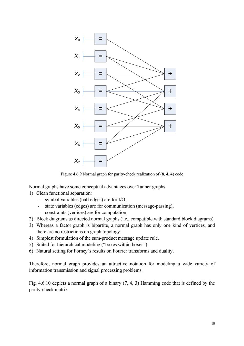
= = + Figure 9 Normal graph for parity-check realization of (8)code Normal graphs have some conceptual advantages over Tanner graphs 1)Clean functional separation: symbol variables (half edges)are for I/O; 、 state variables(edges)are for communication(message-passing): straints(vertic 3)Whereas a factor graph is bipartite,a normal graph has only one kind of vertices,and there are no restrictions on graph topology. 4)Simplest formulation of the sum-product message update rule. 5)Suited for hierarchical modeling("boxes within boxes"). 6)Natural setting for Forey's results on Fourier transforms and duality Therefore,normal graph provides an attractive notation for modeling a wide variety of information transmission and signal processing problems. Fig 4.6.10 depicts a normal graph of a binary(7.4.3)Hamming code that is defined by the parity-check matrix
10 X0 X1 X2 X3 X4 X5 X6 X7 Figure 4.6.9 Normal graph for parity-check realization of (8, 4, 4) code Normal graphs have some conceptual advantages over Tanner graphs. 1) Clean functional separation: - symbol variables (half edges) are for I/O; - state variables (edges) are for communication (message-passing); - constraints (vertices) are for computation. 2) Block diagrams as directed normal graphs (i.e., compatible with standard block diagrams). 3) Whereas a factor graph is bipartite, a normal graph has only one kind of vertices, and there are no restrictions on graph topology. 4) Simplest formulation of the sum-product message update rule. 5) Suited for hierarchical modeling (“boxes within boxes”). 6) Natural setting for Forney’s results on Fourier transforms and duality. Therefore, normal graph provides an attractive notation for modeling a wide variety of information transmission and signal processing problems. Fig. 4.6.10 depicts a normal graph of a binary (7, 4, 3) Hamming code that is defined by the parity-check matrix