第49卷第5期 林 业 科学 Vol.49,No.5 2013年5月 SCIENTIA SILVAE SINICAE May,2013 doi:10.11707/j.1001-7488.20130515 树木位置空间模式建模与预测* 金星姬李凤日'贾炜玮 张连军2 (1.:东北林业大学林学院哈尔滨150040:2.美国纽约州立大学环境科学和林业学院锯拉丘兹NY13210) 摘要:传统的林分生长与收获模型不能为林分和生态系统管理提供准确的空间信息。采用3种配对势函数的 Gibbs点过程模型对美国东北部50块云冷杉样地里树木的空间分布模式进行模拟。该Gibbs模型能够较好地模拟 这50块样地中的82%~84%,但其对完全随机分布和规则分布的样地模拟比对聚集分布的样地模拟效果要好。 使用常用的林分变量如林分密度、公顷断面积、林分平均胸径、平均树高、平均冠幅和冠长建立经验回归模型对 Gbbs模型的2个参数进行预测。结果表明这些回归模型对81%的样地可以得到满意的模拟效果,其中,100%的 完全随机分布样地、71%的规则分布样地和56%的聚集分布样地模拟效果较好。选择3块样地对树木的模拟空间 位置和实际观测位置的相似性进行对比和说明。 关键词:空间点模式;空间点过程:Gibbs模型;Ripley's K--function;马尔可夫链Monte Carlo(MCMC); Metropolis算法;Takacs-Fiksel方法 中图分类号:S711 文献标识码:A 文章编号:1001-7488(2013)05-0110-11 Modeling and Predicting Spatial Patterns of Trees Jin Xingji'Li Fengri'Jia Weiwei'Zhang Lianjun' (1.School of Forestry,Northeast Forestry University Harbin 150040; 2.College of Environmental Science and Forestry.State University of New York (SUNY-ESF)Syracuse,NY13210,USA) Abstract:Traditional forest growth and yield models have been criticized for their inability to provide precise spatial information for forest and ecosystem management.In this study the spatial patterns of trees within 50 spruce-fir plots in the Northeast,USA were modeled by a Gibbs point process model with three pair potential functions.In general,82%-84% of these 50 plots were modeled well by the Gibbs model.However,the complete spatial random CSR)and regular spatial patterns were modeled better than the clustered plots.Further,empirical regression models were developed to predict the two parameters of the Gibbs model using the available stand variables as predictors such as stand density,basal area, mean tree diameter,mean tree height,mean crown length,and mean crown width.The simulation results showed that 81%of the 50 plots were satisfactorily predicted by the empirical regression models.Among them,100%of the CSR plots,71%of the regular plots,and 56%of the clustered plots were predicted well by the empirical regression models. Three example plots were selected to illustrate the similarity between simulated tree locations and observed ones. Key words:spatial point pattern;spatial point process;Gibbs model;Ripley's K-function;Markov Chain Monte Carlo (MCMC);Metropolis algorithm;Takacs-Fiksel method chance success of different species or individuals over 1 Introduction time.The spatial distributions of trees strongly affect Spatial patterns of tree locations in a forest stand competition between neighboring trees,size variability reflect the complex historical and environmental mosaic and distribution,growth and mortality,and crown imposed by initial establishment patterns, structure Kuuluvainen et al.,1987;Kenkel,1988; microenvironment differences,climatic factors, Miller et al.,1989;Hara,1992;Moeur,1993; competing vegetation,management activities,and the Rouvinen et al.,1997;Dovciak et al.,2001 ) Received date:2012-08-06;Revised date:2012-10-12 Foundation project:Supported by the Scientifie Research Funds for Forestry Publie Welfare of China(201004026);Ministry of Education "Overseas Experts and Scholars"project. Corresponding author:Li Fengri. 万方数据
第49卷第5期 2 0 1 3年5月 林 业 科 学 SCIENTIA SILVAE SINICAE VoL 49.No.5 May,2 0 1 3 doi:10.11707/j.1001-7488.20130515 树木位置空间模式建模与预测 金星姬1 李凤日1 贾炜玮1 张连军2 (1.东北林业大学林学院哈尔滨150040;2.美国纽约州立大学环境科学和林业学院锡拉丘兹NYl3210) 摘 要: 传统的林分生长与收获模型不能为林分和生态系统管理提供准确的空间信息。采用3种配对势函数的 Gibbs点过程模型对美国东北部50块云冷杉样地里树木的空间分布模式进行模拟。该Gibbs模型能够较好地模拟 这50块样地中的82%一84%,但其对完全随机分布和规则分布的样地模拟比对聚集分布的样地模拟效果要好。 使用常用的林分变量如林分密度、公顷断面积、林分平均胸径、平均树高、平均冠幅和冠长建立经验回归模型对 Gibbs模型的2个参数进行预测。结果表明这些回归模型对81%的样地可以得到满意的模拟效果,其中,100%的 完全随机分布样地、7t%的规则分布样地和56%的聚集分布样地模拟效果较好。选择3块样地对树木的模拟空间 位置和实际观测位置的相似性进行对比和说明。 关键词: 空间点模式;空间点过程;Gibbs模型;Ripley’S K—function;马尔可夫链Monte Carlo(MCMC); Metropolis算法;Takacs.Fiksel方法 中图分类号:$711 文献标识码:A 文章编号:1001—7488(2013)05—0110—11 Modeling and Predicting Spatial Patterns of Trees Jin Xingji Li Fengri 1 Jia Weiwei Zhang Lianjun2 (1.School of Forestry,Northeast Forestry University Harbin 150040; 2.College ofEnvironmental Science and Forestry,State University ofNew York(SUNY-ESF)Syracuse,NYl3210,USA) Abstract:Traditional forest growth and yield models have been criticized for their inability to provide precise spatial information for forest and ecosystem management.In this study the spatial patterns of trees within 50 spruce·fir plots in the Northeast,USA were modeled by a Gibbs point process model with three pair potential functions.In general,82%一84% of these 50 plots were modeled well by the Gibbs model.However,the complete spatial random(CSR)and regular spatial patterns were modeled better than the clustered plots.Further,empirical regression models were developed to predict the two parameters of the Gibbs model using the available stand variables as predictors such as stand density,basal area, mean tree diameter,mean tree height,mean crown length,and mean crown width.The simulation resuhs showed that 8l%of the 50 plots were satisfactorily predicted by the empirical regression models.Among them.100%of the CSR plots,7 1%of the regular plots,and 56%of the clustered plots were predicted well by the empirical regression models. Three example plots were selected to illustrate the similarity between simulated tree locations and observed ones. Key words: spatial point pattern;spatial point process;Gibbs model;Ripley’S K—function;Markov Chain Monte Carlo (MCMC);Metropolis algorithm;Takacs—Fiksel method 1 Introduction Spatial patterns of tree locations in a forest stand reflect the complex historical and environmental mosaic imposed by initial establishment patterns, microenvironment differences, climatic factors, competing vegetation,management activities,and the chance success Of difierent species or individuals over time.The spatial distributions of trees strongly affect competition between neighboring trees,size variability and distribution,growth and mortality,and crown structure(Kuuluvainen et a1.,1987;Kenkel,1988; Miller et a1.,1989;Hara,1992;Moeur,1993; Rouvinen et a1.,1997;Dovciak et a1.,2001). Received date:2012一08—06;Revised date:2012—10—12, Foundation project:Supported by the Scientific Research Funds for Forestry Public Welfare of China(201004026);Ministry of Education“Overseas Expels and Scholars”project. $Corresponding author:Li Fen96. 万方数据
第5期 金星姬等:树木位置空间模式建模与预测 111 Furthermore,the spatial patterns at tree-scale have One such model is the Gibbs point process model large influences on system-level and community-level or pairwise interaction process model )which properties of ecosystem functions (Pacala et al.,1995; assumes the interaction between two events (e.g., Friedman et al.,2001).In general,positive spatial trees)depends on the relative location of them.It dependence among neighboring trees is mainly due to originates from statistical physics Wood,1968; the effects of the micro-site,whereas inter-tree Landau et al,1980)and has been intensively used in competition tends to create negative spatial dependence spatial statistics (Stoyan et al.,1987;Ogata et al, among neighboring trees Fox et al.,2001). 1981;1984;1985;Diggle et al.,1994).The Gibbs Spatial point pattern analysis is commonly used to point process model with pair potential functions is a study the distributions of the horizontal spacing among class of models for point patterns exhibiting interactions trees within a region of interest.The objective of between the events.These models have been applied spatial point pattern analysis is to measure how in forestry and ecological studies due to their great individual trees are located with respect to each other flexibility and realism in modeling different spatial by using quantitative characteristics and to describe the point patterns (Tomppo,1986;Penttinen et al.,1992; "laws"regulating the locations with mathematical Stoyan et al.,1998;Sarkka et al.,1998;Stoyan et al., models Diggle,1983;Tomppo,1986;Pretzsch, 2000). 1997).There are three fundamental spatial point Different methods have been developed to estimate patterns:complete spatial randomness (CSR ) the parameters of the pair potential functions.Diggle et regularity,and clustering.This classification is over- al.(1994)summarizes three general methods,namely simplified,but useful at an early stage of spatial approximations of maximum likelihood,maximum analysis.It is also helpful to formulate a model for the pseudo-likelihood,and Takacs-Fiksel method.These underlying spatial point process Diggle,1983).A methods can be routinely used in applications and there spatial point pattern is the realization of a spatial point are no restrictions on the parametric form of the pair process (Cressie,1993).Once the spatial point potential functions Tomppo,1986;Stoyan et al., patterns are recognized,it is desirable to fit appropriate 1987;Jensen et al.,1991). point process models to the spatial patterns in order to Spruce-fir stands in the Northeast,USA are understand the mechanisms generating the patterns and traditionally important resources for timber production. to perform analyses of goodness-of-fit for the models. Forest managers and researchers have developed a Detailed review on spatial point process models can be variety of tools for managing these stands.These tools found in the literature (Cressie,1993;Tomppo, include stocking charts and stand density management 1986;Stoyan et al.,2000). diagrams for the pure and mixed softwood stands in the The spatial point process generating CSR is called region (Solomon et al.,2002).However,very little a homogeneous Poisson process,such that the number spatial information is available for these stands to date. of events realized by this process 1)follow a Poisson The objectives of this research were 1)to explore the distribution with mean equal to AA,where A is the spatial structures of the spruce-fir softwood stands in density or intensity of events (e.g.,trees)and A is the Northeast,USA,2)to fit the Gibbs point process the area of the region A;and 2)are independent model with three pair potential functions to the spatial random samples from the uniform distribution on A patterns of trees within the stands,and 3)to develop (Cressie,1993;Diggle,1983).Intuitively,CSR empirical regression models for predicting the means that events are equally likely to occur anywhere parameters of the Gibbs point process model using within A and that events do not interact with each other available stand variables. (Cressie,1993).The homogeneous Poisson point 2 Data and methods process usually serves as a null model Stoyan et al., 2000).If the null model is rejected,more complicated 2.1 Data models are necessary to be tested (Tomppo,1986). Fifty (50)plots were collected from the even- 万方数据
第5期 金星姬等:树木位置空间模式建模与预测 111 Furthermore,the spatial patterns at tree-scale have large influences on system·level and community.1evel properties of ecosystem functions(Pacala et a1.,1 995; Friedman et a1.,200 1).In general,positive spatial dependence among neighboring trees is mainly due to the effects of the micro—site,whereas inter.tree competition tends to create negative spatial dependence among neighboring trees(Fox et a1.,2001). Spatial point pattern analysis is commonly used to study the distributions of the horizontal spacing among trees within a region of interest.The objective of spatial point pattern analysis is to measure how individual trees are located with respect to each other by using quantitative characteristics and to describe the “laws”regulating the locations with mathematical models(Diggle,1983;Tomppo,1986;Pretzsch, 1 997).There are three fundamental spatial point patterns: complete spatial randomness(CSR), regularity,and clustering.This classification is over. simplified,but useful at an early stage of spatial analysis.It is also helpful to formulate a model for the underlying spatial point process(Diggle,1983).A spatial point pattern is the realization of a spatial point process(Cressie,1 993).Once the spatial point patterns are recognized,it is desirable to fit appropriate point process models to the spatial patterns in order to understand the mechanisms generating the patterns and to perform analyses of goodness—of—fit for the models. Detailed review on spatial point process models can be found in the literature(Cressie,1 993;Tomppo, 1986;Stoyan et a1.,2000). The spatial point process generating CSR is called a homogeneous Poisson process,such that the number of events realized by this process 1)follow a Poisson distribution with mean equal to A A l,where A is the density or intensity of events(e.g.,trees)and A|is the area of the region A;and 2)are independent random samples from the uniform distribution on A (Cressie,1993;Diggle,1983).Intuitively,CSR means that events are equally likely to occur anywhere within A and that events do not interact with each other (Cressie,1 993).The homogeneous Poisson point process usually serves as a null model(Stoyan et a1., 2000).If the null model is models are necessary to be rejected,more complicated tested(Tomppo,1986). One such model is the Gibbs point process model (or pairwise interaction process model),which assumes the interaction between two events(e.g., trees)depends on the relative location of them.It originates from statistical physics(Wood,1 968; Landau et a1.,1 980)and has been intensively used in spatial statistics(Stoyan et a1.,1987;Ogata et a1., 1981;1984;1985;Diggle et a1.,1994).The Gibbs point process model with pair potential functions is a class of models for point patterns exhibiting interactions between the events.These models have been applied in forestry and ecological studies due to their great flexibility and realism in modeling different spatial point patterns(Tomppo,1 986;Penttinen et a1.,1 992; Stoyan et a1.,1998;Sarkka et a1.,1998;Stoyan et a1., 2000). Different methods have been developed to estimate the parameters of the pair potential functions.Diggle et a1.(1 994)summarizes three general methods,namely approximations of maximum likelihood, maximum pseudo—likelihood,and Takacs-Fiksel method.These methods can be routinely used in applications and there are no restrictions on the parametric form of the pair potential functions(Tomppo,1986;Stoyan et a1., 1987;Jensen et a1.,1991). Spruce-fir stands in the Northeast,USA are traditionally important resources for timber production. Forest managers and researchers have developed a variety of tools for managing these stands.These tools include stocking charts and stand density management diagrams for the pure and mixed softwood stands in the region(Solomon et a1.,2002).However,very little spatial information is available for these stands to date. The objectives of this research were 1)to explore the spatial structures of the spruce—fir softwood stands in the Northeast,USA,2)to fit the Gibbs point process model with three pair potential functions to the spatial patterns of trees within the stands,and 3)to develop empirical regression models for predicting the parameters of the Gibbs point process model using avai】ab】e stand variables. 2 Data and methods 2.1 Data Fifty(50)plots were collected from the even- 万方数据
112 林业科学 49卷 aged spruce-fir forests in northwestern Maine,USA, trees.The forest plot A is a sampling window within a located in the region between 69 W and 71 W in much larger forest region.Therefore,the events longitude,between 45 N and 46.5 N in latitude,and (trees)are the points of a partial realization of a between 750 m and I 200 m in elevation planar point process within A.For the patterns of N (Kleinschmidt et al.,1980).The plot size ranged from trees in a bounded region A,the pairwise interaction 0.002 5 to 0.02 hm2.The shapes of the plots were processes (i.e.,pair-potential processes)are suitable mostly square with a few rectangular.In each plot,the stochastic models.The joint density for these processes position of each tree over 1.37 m in height was mapped generally takes the form of Li et al,2007).In these plots balsam fir (Abies )=A”。 balsamea)and red spruce (Picea rubens)accounted e即{-A(Ix-xID}, for about 95%of total number of trees and 94%of (1) total volume.Other minor species included black where is the Euclidean distance between trees i cherry (Prunus serotina),eastern white pine (Pinus and j,B is a parameter determining the intensity of the strobus),white spruce Picea glauca),black spruce process,()is a pair potential function,and C is a Picea mariana),and other hardwoods.Tree diameter normalizing constant to make f(x)a density depending at breast height (DBH),total height,crown length on B and中(·). (top to the base of crown),and average crown width The homogeneous Gibbs point process is a special were recorded for each tree (Solomon et al,2002). case of pairwise interaction processes.It is The numbers of trees in each plot ranged from 12 to characterized by the potential functionΦ(·)and 109.Mean tree diameters were from 2.2 to 19.2 cm another parameter a =-log(B).Although the explicit and mean tree total heights were from 2.7 to 17.1 form of the distribution is hard to obtain,the following m (Tab.1). relationship holds for a homogeneous Gibbs point process Diggle et al.,1994) Tab.1 Summary statistics of the stand AE[Z(X)]= variables across the 50 plots Stand variables Mean Std.Min.Max. Number of trees per plot 34.4 17.7 12 109 Efz(X)exp[-a-((2) Stand density/(tree.m2) 0.61 0.54 0.18 2.52 where A is the density of events,Eo is the expectation Stand basal area/(m2.hm-2)50.2 14.3 10.0 79.6 Stand mean DBH/cm 11.53.9 2.2 19.2 with respect to the Palm distribution of the process,E Stand mean height/m 11.63.7 2.7 17.1 is the expectation,and Z(X)is any random function Stand mean crown length/m 4.41.5 1.6 8.4 of the process where X includes all events of the Stand mean crown width/m 1.I 0.3 0.5 1.9 process in the whole plane.For a strict definition of Using the methods of refined nearest neighbor Palm distribution,see Stoyan et al.(1987),Tomppo statistic,Ripley's K-function (Ripely,1976)analysis (1986)and Cressie (1993). and pair correlation function analysis,24 plots were However,when it is conditional on the number of classified as completely spatial random (CSR)point points N,Gibbs distribution can be expressed as pattern,17 plots as regular point pattern,and 9 plots as clustered point pattern out of the 50 plots (Li et al., )=2ep{-会Ax.-XD}.3) where Z is the normalizing constant in the form of 2007).The classification was used as the basis for modeling the spatial patterns in this study z=ep-合点X,-XD],d 2.2 Methods The pair potential function()can be interpreted as 2.2.1 Theoretical background of Gibbs model followings:(d)>0 indicates that the probability pairwise interaction process model)Suppose the density for inter-event distance d is lower than that spatial point pattern in a mapped forest plot A has N under Poisson process and,thus,there is repulsion at events (trees).Denote=X =(u:,v)EA:i=1, distance d;(d)<0 indicates that the probability 2,..,N as the set of coordinates (u:,v)of the density for inter-event distance d is higher than that 万方数据
112 林业科学 49卷 aged spruce—fir forests in northwestern Maine,USA, located in the region between 69。W and 7 1。W in longitude,between 45。N and 46.5。N in latitude,and between 750 m and l 200 m in elevation (Kleinschmidt et a1.,1980).The plot size ranged from 0.002 5 to 0.02 hm2.The shapes of the plots were mostly square with a few rectangular.In each plot,the position of each tree over 1.37 m in height was mapped (Li et a1.,2007).In these plots batsam fir(Abies balsamea)and red spruce(Picea rubens)accounted for about 95%of total number of trees and 94%of total volume.Other minor species included black cherry(Prunus serotina),eastern white pine(Pinus strobus),white spruce(Picea glauca),black spruce (Picea mariana),and other hardwoods.Tree diameter at breast height(DBH),total height,crown length (top to the base of crown),and average crown width were recorded for each tree(Solomon et a1.,2002). The numbers of trees in each plot ranged from 1 2 to 109.Mean tree diameters were from 2.2 to 19.2 am and mean tree total heights were from 2.7 to 17.1 m(Tab.1). Tab.1 Summary statistics of the stand variables across the 50 plots Stand variables Mcan Std. Min. Max. Number oftrees per plot 34.4 17.7 12 109 Stand density/(tree·m一2)0.61 0.54 0.18 2.52 Stand basal area/(m2.hm一2) 50.2 14.3 10.0 79.6 Stand mean DBH/cm 11.5 3.9 2.2 19.2 Stand mean height/m 11.6 3.7 2.7 17.1 Stand mean crown length/m 4.4 1.5 1.6 8.4 Stand mean crown width/m 1.1 0.3 0.5 1.9 Using the methods of refined nearest neighbor statistic.Ripley’s K-function(Ripely,1 976)analysis and pair correlation function analysis,24 plots were classified as completely spatial random(CSR)point pattern,1 7 plots as regular point pattern,and 9 plots as clustered point pattern out of the 50 plots(Li et a1., 2007).The classification was used as the basis for modeling the spatial patterns in this study. 2.2 Methods 2.2.1 Theoretical background of Gibbs model (pairwise interaction process model) Suppose the spatial point pattern in a mapped forest plot A has N events(trees).Denote X={X。=(Mi,口。)∈A:i=1, 2,…,Ⅳ}as the set of coordinates(Mi,u。)of the trees.The forest plot A is a sampling window within a much larger forest region.Therefore,the events (trees)are the points of a partial realization of a planar point process within A.For the patterns of N trees in a bounded region A,the pairwise interaction processes(i.e.,pair—potential processes)are suitable stochastic models.The joint density for these processes generally takes the form of 州=篇唧{-乏。三驯l xi.Xj∽), (1) where㈩I is the Euclidean distance between trees i and j,8 is a parameter determining the intensity of the process,多(·)is a pair potential function,and C is a normalizing constant to make八z)a density depending on口and中(·). The homogeneous Gibbs point process is a special case of pairwise interaction processes. It is characterized by the potential function中(‘)and another parameter a=一log(f1).Although the explicit form of the distribution is hard to obtain,the following relationship holds for a homogeneous Gibbs point process(Diggle et a1.,1994) AE“Z(X)]= E{z(x)exp[一a一萎中(…I)])’(2) where A is the density of events,Eo is the expectation with respect to the Palm distribution of the process,E is the expectation,and Z(X)is any random function of the process where X includes a11 events of the process in the whole plane.For a strict definition of Palm distribution,see Stoyan et a1.(1987),Tomppo (1986)and Cressie(1993). However.when it is conditional on the number of points N,Gibbs distribution can be expressed as 以并)=Z-1exp{-∑∑西(1IXi一划)},(3) where Z is the normalizing constant in the form of z=exp[一乏。三中(IIX;一圳h,…,d‰· The pair potential function多(·)can be interpreted as followings:中(d)>0 indicates that the probability density for inter.event distance d is lower than that under Poisson process and,thus,there is repulsion at distance d;中(d)<0 indicates that the probability density for inter.event distance d is higher than that 万方数据
第5期 金星姬等:树木位置空间模式建模与预测 113 under Poisson process.Thus,there is attraction at length of parameter vector (a,) distance d;and (d)=0 indicates a Poisson process. There is no agreed rule for choosing the function 2.2.2 Pair potential functions The pair potential Z.However,if the test function Z:is chosen to be function ()can be parameterized in various forms. equal to N()Diggle et al,1994),which is the In this study,three parametric models were adopted. number of events i with:-X‖≤rk,where X,(U= The first one is called Very-Soft-Core (VSC)pair 1,2,...,L)is the jth randomly chosen testing point, potential function (Ogata et al,1984): the left side of equation (2)can be estimated as Φ(r)=-lgi1-exp[-(r/6)2]},(4) i.(a,0)=A2K(r), (8) where 6 is a scaling parameter.For the VSC pair where K(r)is Ripley's K-function (Ripley,1976; potential function,the range of interaction is infinite 1977).The right side of equation (2)can be for all distance r.The second one is called Diggle's estimated as pair potential function that has the following form Diggle et al.,1994): 元(e,9)=它N() ()=-lg(1-[1-(/8)2]2),fr≤; N (9) 0, if rx6. exp-&-∑Φ(Ix-X,I)] =1 (5) The choices of L,m and r.are arbitrary although where the scaling parameter 6 defines the range of different values can be tried and compared.For the interaction.The third one is called Ogata and data used in this study,we set the constants as Tanemura's pair potential function (Ogata et al., follows:1)L=2N because we wanted to ensure that 1985): there were enough random points surrounding a tree, (r)=-lg(1+[r(r/8)-1] and 2)m =30 and r=0.Ik which made the exp[-(r/8)2]),r≥0,8>0, (6) maximum value 3.0 m)because we wanted there to be where the scaling parameter 6 defines the range of enough but not too many trees within the plot which are interaction.Notice that equation(4)is a special case of considered interacting with each other. equation(6)when the parameter 7=0.For equation The optimization of equation(7)was performed (5),(r)=0 when r=6 representing the Poisson using a direct search polytope algorithm one available process.For equation(6),(r)=0 when T =5/r, subroutine is the UMPOL in the IMSL Math Library of which represents the Poisson process. Fortran PowerStation 4.0 C 1994-95 Microsoft 2.2.3 Parameter estimation method One of the Corporation).Details of the polytope algorithm can be methods for estimating the parameters of the pair found in the literature (Nelder et al.,1965;Gill et al., 1981). potential functions is the Takacs-Fiksel method (Diggle et al.,1994).It is based on the fundamental 2.2.4 Edge corrections Typically,the study relationship in equation (2).Suppose is the regions would be the sampled plots within a forest stand.Each of these plots covers only a part of the parameter vector of a pair potential function0=8 for entire spatial pattern.Interactions can only be the potential functions(4)and(5)or =(7,)for the potential function(6)).If a series of test functions Z observed among the trees within a plot,while interactions are unobserved between the trees within (k=1,2,...,m)are chosen to estimate both sides of the plot and the trees outside the plots.It is known as equation(2)(denoting the left side as L(a,0)and the edge or boundary effect.If no correction is taken the right side as R(a,0)),the sum of squared for the boundary effect in the point pattern analysis, differences of both sides can be minimized to estimate the estimation of the interactions is biased.In the the model parameters (a,0)as, previous study Li et al.,2007),the toroidal edge S(a,6)=∑[i(a,0)-(a,0)]2,(7) correction method was proven to be simple and satisfactory compared with other available edge where m is some arbitrary number no less than the correction methods such as buffer zone,border 万方数据
第5期 金星姬等:树木位置空间模式建模与预测 113 —————————————————————————————————————————————————一一 under Poisson process.Thus,there is attraction at distance d;and中(d)=0 indicates a Potsson Drocess. 2.2.2 Pair potential functions The pair potential function中(·)can be parameterized in various forms. In this study,three parametric models were adopted. The first one is called Very.Soft.Core(VSC)pair potential function(Ogata et a1.,1 984): 中(r)=一lg{1一exp[一(r俗)2] where 6 is a scaling parameter.For the VSC Dair potential function,the range of interaction is innnite for all distance,.The second one is called Diggle’s pair potential function that has the foliowing form (Diggle et a1.,1994): 西(r):r 19(1~[1一(r/a)2]2),if r≤6; 【 o, if r>占. (5) where the scaling parameter 6 defines the range of interaction.The third one is called Ogata and Tanemura’8 pair potential function(Ogata et a1.. 1985): 西(r)=一lg(1+[丁(r/8)一1] exp[一(r/8)2]),r≥0,6>0, (6) where the scaling parameter 6 defines the range of interaction.Notice that equation(4)is a special case of equation(6)when the parameter 7.=0.For equation (5),中(r)=-0 when r=6 representing the Poisson process.For equation(6),西(r)-=0 when丁=6/r. which represents the Poisson process. 2.2.3 Parameter estimation method 0ne of the methods for estimating the parameters of the pair potential functions is the Takacs—Fiksel method(Diggle et a1.,1994). It is based on the fundamental relationship in equation(2).Suppose 0 is the parameter vector of a pair potential function[0=6 for the potential functions(4)and(5)or 0=(下,∞for the potential function(6)].If a series of test functions Z‘ (k=1,2,…,m)are chosen to estimate both sides of equation(2)(denoting the left side as L^(ot,0)and the right side as R^(ot,0)),the sum of squared differences of both sides can be minimized to estimate the model parameters(ot,0)as, 5(a,口)=∑哦(a,日)一壶。(a,∽]2,(7) t:1 where m is some arbitrary number no less than the length of parameter vector(a,0). There is no agreed rule for choosing the function ZI.However, if the test function Z‘is chosen to be equal to%(r女)(Diggle et a1.,1994),which is the number of events i with lIX。一x,II≤k,where x,(,= 1,2,…,L)is thejth randomly chosen testing point. the left side of equation(2)can be estimated as L^(o/,0) where K(r^)is Ripley’s 1977).The right side estimated as =A 2K(0), (8) K—function(Ripley,1 976; of equation(2)can be 交如∽=÷萎L_㈠) exp[一a一萎4(IIx。一训】. (9) The choices of£,m and^are arbitrary although different values can be tried and cornpared.For the data used in this study, we set the constants as follows:1)L=2N because we wanted to ensure that there were enough random points surrounding a tree, and 2)m=30 and o=0.1七(which made the maximum value 3.0 m)because we wanted there to be enough but not too many trees within the plot which are considered interacting with each other. The optimization of equation(7)was performed using a direct search polytope algorithm(one available subroutine is the UMPOL in the IMSL Math Library of Fortran PowerStation 4.0 c|C 1 994—95 Microsoft Corporation).Details of the polytope algorithm can be found in the literature(Nelder et a1.,1 965;Gill et of.. 1981). 2.2.4 Edge corrections Typically,the study regions would be the sampled plots within a forest stand.Each of these plots covers only a part of the entire spatial pattern. Interactions can only be observed among the trees within a plot, while interactions are unobserved between the trees within the plot and the trees outside the plots.It is known as the edge or boundary effect.If no correction is taken for the boundary effect in the point pattern analysis. the estimation of the interactions is biased.In the previous study(Li et a1.,2007),the toroidal edge correction method was proven to be simple and satisfactory compared with other available edge correction methods such as bufier zone. borde。 万方数据
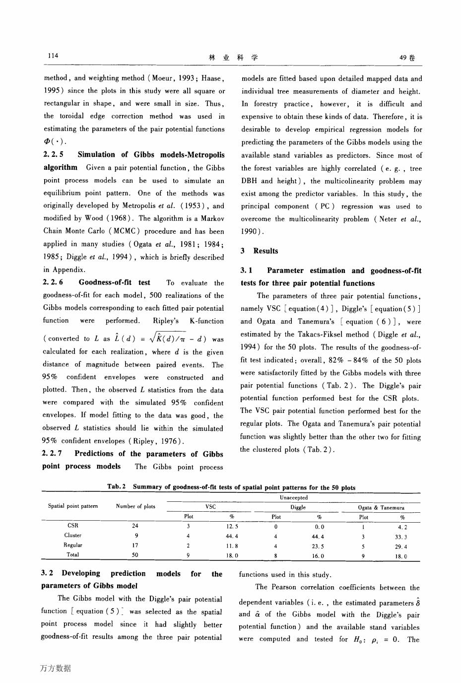
114 林业科学 49卷 method,and weighting method Moeur,1993;Haase, models are fitted based upon detailed mapped data and 1995)since the plots in this study were all square or individual tree measurements of diameter and height. rectangular in shape,and were small in size.Thus, In forestry practice,however,it is difficult and the toroidal edge correction method was used in expensive to obtain these kinds of data.Therefore,it is estimating the parameters of the pair potential functions desirable to develop empirical regression models for 中(). predicting the parameters of the Gibbs models using the 2.2.5 Simulation of Gibbs models-Metropolis available stand variables as predictors.Since most of algorithm Given a pair potential function,the Gibbs the forest variables are highly correlated (e.g.,tree point process models can be used to simulate an DBH and height),the multicolinearity problem may equilibrium point pattern.One of the methods was exist among the predictor variables.In this study,the originally developed by Metropolis et al.(1953),and principal component PC)regression was used to modified by Wood (1968).The algorithm is a Markov overcome the multicolinearity problem (Neter et al., Chain Monte Carlo (MCMC)procedure and has been 1990). applied in many studies (Ogata et al.,1981;1984; 3 Results 1985;Diggle et al.,1994),which is briefly described in Appendix. 3.1 Parameter estimation and goodness-of-fit 2.2.6 Goodness-of-fit test To evaluate the tests for three pair potential functions goodness-of-fit for each model,500 realizations of the The parameters of three pair potential functions, Gibbs models corresponding to each fitted pair potential namely VSC equation(4)],Diggle's equation(5)] function were performed.Ripley's K-function and Ogata and Tanemura's equation (6)],were converted to L as i(d)=v(d)/i-d)was estimated by the Takacs-Fiksel method (Diggle et al., calculated for each realization,where d is the given 1994)for the 50 plots.The results of the goodness-of- distance of magnitude between paired events.The fit test indicated:overall,82%-84%of the 50 plots 95%confident envelopes were constructed and were satisfactorily fitted by the Gibbs models with three plotted.Then,the observed L statistics from the data pair potential functions (Tab.2).The Diggle's pair were compared with the simulated 95%confident potential function performed best for the CSR plots. envelopes.If model fitting to the data was good,the The VSC pair potential function performed best for the observed L statistics should lie within the simulated regular plots.The Ogata and Tanemura's pair potential 95%confident envelopes Ripley,1976). function was slightly better than the other two for fitting 2.2.7 Predictions of the parameters of Gibbs the clustered plots (Tab.2). point process models The Gibbs point process Tab.2 Summary of goodness-of-fit tests of spatial point patterns for the 50 plots Unaccepted Spatial point pattern Number of plots VSC Diggle Ogata Tanemura Plot Plot Plot % CSR 24 3 12.5 0 0.0 4.2 Cluster 9 4 44.4 4 44.4 3 33.3 Regular 17 2 11.8 4 23.5 J 29.4 Total 50 9 18.0 8 16.0 9 18.0 3.2 Developing prediction models for the functions used in this study. parameters of Gibbs model The Pearson correlation coefficients between the The Gibbs model with the Diggle's pair potential dependent variables (i.e.,the estimated parameters 8 function equation(5)was selected as the spatial and a of the Gibbs model with the Diggle's pair point process model since it had slightly better potential function)and the available stand variables goodness-of-fit results among the three pair potential were computed and tested for Ho:p=0.The 万方数据
114 林业科学 49卷 method,and weighting method(Moeur,1993;Haase, 1 995)since the plots in this study were all square or rectangular in shape,and were small in size.Thus, the toroidal edge correction method was used in estimating the parameters of the pair potential functions 西(·). 2.2.5 Simulation of Gibbs models-Metropolis algorithm Given a pair potential function,the Gibbs point process models can be used to simulate an equilibrium point pattern.One of the methods was originally developed by Metropolis et a1.(1953),and modified by Wood(1 968).The algorithm is a Markov Chain Monte Carlo(MC MC)procedure and has been applied in many studies(Ogata et a1.,1981;1984; 1 985;Diggle et at.,1 994),which is briefly described in Appendix. 2.2.6 Goodness-of-fit test To evaluate the goodness—of-fit for each model,500 realizations of the Gibbs models corresponding to each fitted pair potential function were performed. Ripley’s K—function (convened to L as£(d)= r■————~ √K(d)/竹一d) was calculated for each realization,where d is the given distance of magnitude between paired events.The 95% confident envelopes were constructed and plotted.Then,the observed L statistics from the data were compared with the simulated 95%confident envelopes.If model fitting to the data was good,the observed L statistics should lie within the simulated 95%confident envelopes(Ripley,1 976). 2.2.7 Predictions of the parameters of Gibbs point process models The Gibbs point process models are fitted based upon detailed mapped data and individual tree measurements of diameter and height. In forestry practice,however,it is difficult and expensive to obtain these kinds of data.Therefore,it is desirable to develop empirical regression models for predicting the parameters of the Gibbs models using the available stand variables as predictors.Since most of the forest variables are highly correlated(e.g.,tree DBH and height),the muhicolinearity problem may exist among the predictor variables.In this study,the principal component(PC)regression was used to overcome the muhicolinearity problem(Neter et a1., 1990) 3 Results 3·1 Parameter estimation and goodness-of·fit tests for three pair potential functions The parameters of three pair potential functions, namely VSC[equation(4)],Diggle’s[equation(5)] and Ogata and Tanemura’s[equation(6)],were estimated by the Takacs·Fiksel method(Diggle et a1., 1994)for the 50 plots.The results of the goodness—of— fit test indicated:overall,82%一84%of the 50 plots were satisfactorily fitted by the Gibbs models with three pair potential functions(Tab.2).The Diggle’s pair potential function performed best for the CSR plots. The VSC pair potential function performed best for the regular plots.The Ogata and Tanemura’s pair potential function was slightly better than the other two for fitting the clustered plots(Tab.2). Tab.2 Summary of goodness-of—fit tests of spatial point patterns for the 50 plots Unaeeepted Spatial point pattern Number of plots VSC Diggle Ogata&Tanemura Plot %Plot %Plot % CSR 24 3 12.5 0 0.0 1 4.2 Cluster 9 4 44.4 4 44.4 3 33,3 Regular 17 2 11.8 4 23.5 5 29.4 Total 50 9 18.0 8 16.0 9 18.0 3.2 Developing prediction models for the parameters of Gibhs model The Gibbs model with the Diggle’s pair potential function[equation(5):was selected as the spatial point process model since it had slightly better goodness。。of—fit results among the three pair potential functions used in this study. The Pearson correlation coefficients between the dependent variables(i.e..the estimated parameters 6 and a of the Gibbs model with the Diggte’s pair potential function)and the available stand variables were computed and tested for Ho:P。=0.The 万方数据