CHAPTER ELEVEN Application of IS-LM Model macroeconomics N.Gregory Mankiw College of Management,HUST
macroeconomics N. Gregory Mankiw CHAPTER ELEVEN Application of IS-LM Model macro College of Management, HUST
Learning objectives In Chapter 11,we will use the IS-LM model to see how policies and shocks affect income and the interest rate in the short run when prices are fixed derive the aggregate demand curve explore various explanations for the Great Depression CHAPTER 11 Aggregate Demand ll slide 1
CHAPTER 11 Aggregate Demand II slide 1 Learning objectives ▪ In Chapter 11, we will use the IS-LM model to – see how policies and shocks affect income and the interest rate in the short run when prices are fixed – derive the aggregate demand curve – explore various explanations for the Great Depression

Context 1.Explaining fluctuations with IS-LM model 1.1 Policy analysis with IS-LM model 1.2 Interaction between monetary fiscal policy 1.3 Shocks in IS-LM model 2.IS-LM as a theory of aggregate demand 2.1 IS-LM model and aggregate demand 2.2 IS-LM model in short run and long run 3.The Great Depression 4,Chapter summary CHAPTER 11 Aggregate Demand ll slide 2
CHAPTER 11 Aggregate Demand II slide 2 Context 1. Explaining fluctuations with IS-LM model 1.1 Policy analysis with IS-LM model 1.2 Interaction between monetary & fiscal policy 1.3 Shocks in IS-LM model 2. IS-LM as a theory of aggregate demand 2.1 IS-LM model and aggregate demand 2.2 IS-LM model in short run and long run 3. The Great Depression 4. Chapter summary
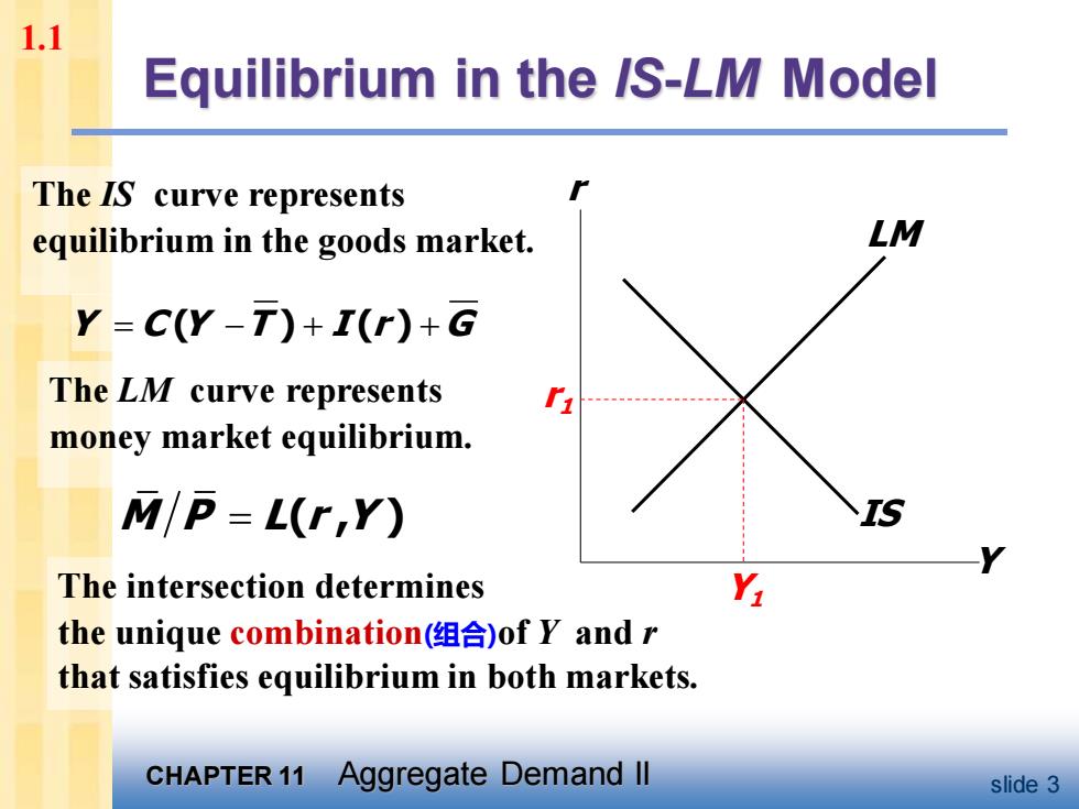
1.1 Equilibrium in the /S-LM Model The IS curve represents equilibrium in the goods market. LM Y=C(Y-T)+I(r)+G The LM curve represents money market equilibrium. M/P=L(r,Y) The intersection determines the unique combination(组合)of Y and r that satisfies equilibrium in both markets. CHAPTER 11 Aggregate Demand Il slide 3
CHAPTER 11 Aggregate Demand II slide 3 The intersection determines the unique combination(组合)of Y and r that satisfies equilibrium in both markets. The LM curve represents money market equilibrium. Equilibrium in the IS-LM Model The IS curve represents equilibrium in the goods market. Y C Y T I r G = − + + ( ) ( ) M P L r Y = ( , ) IS Y r LM r1 Y1 1.1
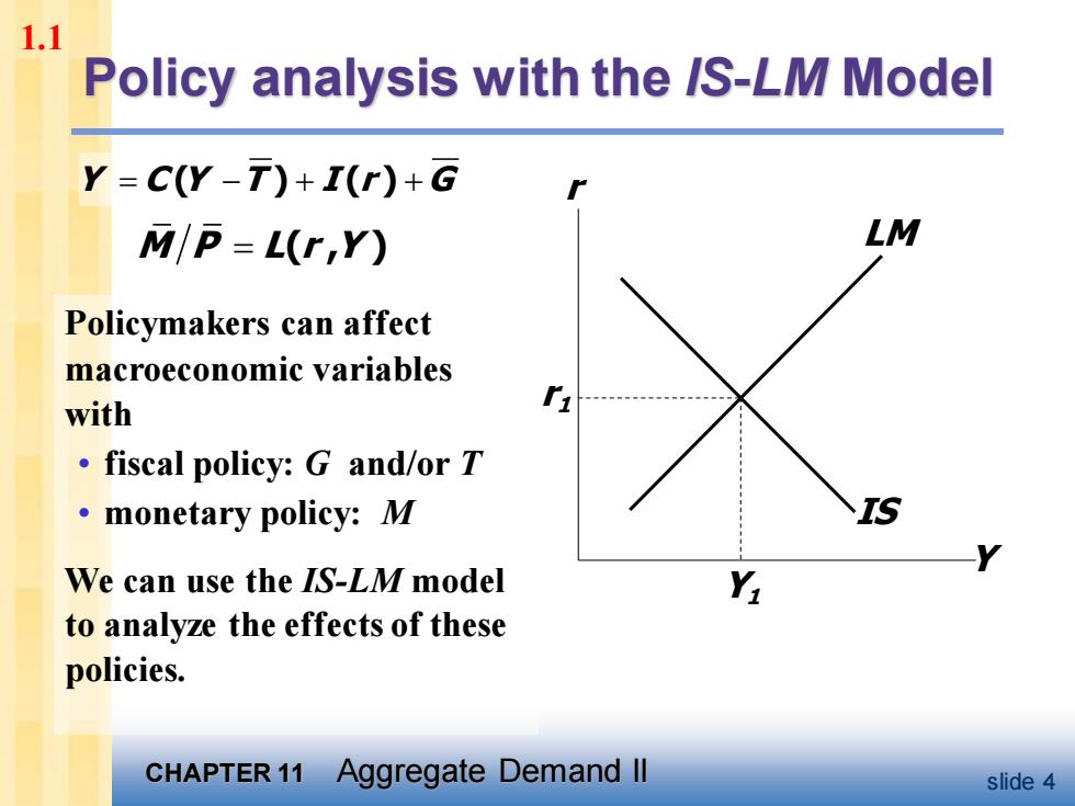
1.1 Policy analysis with the /S-LM Model Y=C(Y-T)+I(r)+G M/P=L(r,Y) LM Policymakers can affect macroeconomic variables with fiscal policy:G and/or T 。monetary policy:.M We can use the IS-LM model to analyze the effects of these policies. CHAPTER 11 Aggregate Demand ll slide 4
CHAPTER 11 Aggregate Demand II slide 4 Policy analysis with the IS-LM Model Policymakers can affect macroeconomic variables with • fiscal policy: G and/or T • monetary policy: M We can use the IS-LM model to analyze the effects of these policies. Y C Y T I r G = − + + ( ) ( ) M P L r Y = ( , ) IS Y r LM r1 Y1 1.1