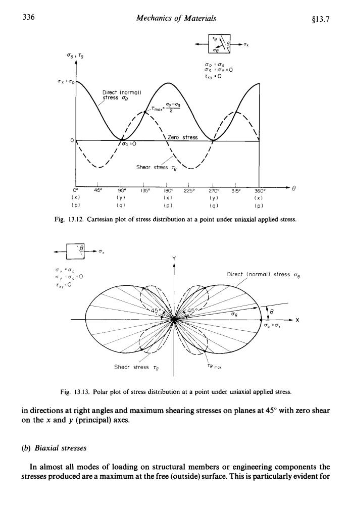
336 Mechanics of Materials §13.7 Ce,Ta 00=可满 0g=gy里0 Try =0 Direct (normol) stress oe 2 0 Zero stress /0g=0 Shear stress Te 45 90° 135°180° 225°2703159. 3560° (×) (y) (x) (y) (x】 (p) (g) (p】 (q】 (p】 Fig.13.12.Cartesian plot of stress distribution at a point under uniaxial applied stress. 0x g,50, Gy=Ga0 Direct (normal)stress g Txy0 459 6 8 X e0, Shear stress Ta Fig.13.13.Polar plot of stress distribution at a point under uniaxial applied stress. in directions at right angles and maximum shearing stresses on planes at 45 with zero shear on the x and y (principal)axes. (b)Biaxial stresses In almost all modes of loading on structural members or engineering components the stresses produced are a maximum at the free (outside)surface.This is particularly evident for
336 Mechanics of Materials $13.7 re I up =ux uq =uy =o r,, :O 1 1 1 I 1 I I O0 45" 90" 135' 180" 225' 270" 315' ? 3"8 IX) (Y) (X) (Y) (X) (P) (q) (P) (q) (PI Fig. 13.12. Cartesian plot of stress distribution at a point under uniaxial applied stress. Y Direct (normal) stress us / X Shear stress ro Fig. 13.13. Polar plot of stress distribution at a point under uniaxial applied stress. in directions at right angles and maximum shearing stresses on planes at 45" with zero shear on the x and y (principal) axes. (b) Biaxial stresses In almost all modes of loading on structural members or engineering components the stresses produced are a maximum at the free (outside) surface. This is particularly evident for

s13.7 Complex Stresses 337 the cases of pure bending or torsion as shown by the stress diagrams of Figs.4.4 and 8.4, respectively,but is also true for other more complex combined loading situations with the major exception of direct bearing loads where maximum stress conditions can be sub-surface. Additionally,at free surfaces the stress normal to the surface is always zero so that the most severe stress condition often reduces,at worst,to a two-dimensional plane stress system within the surface of the component.It should be evident,therefore that the biaxial stress system is of considerable importance to practical design considerations. The Cartesian plot of a typical bi-axial stress state is shown in Fig.13.14 whilst Fig.13.15 shows the polar plot of stresses resulting from the bi-axial stress system present on the surface of a thin cylindrical pressure vessel for which p=o and a=o=to with txy=0. c6,8 Direct (normal)stress 6 Mean stress I0p+0a)=2l0,+oy Tmx乞(p-ga Shear stress Tg 45 90 1359 1809 2259.1270° 315360 (y (y) (x】 《P (q】 (p) (q) Fig.13.14.Cartesian plot of stress distribution at a point under a typical biaxial applied stress system. It should be noted that the whole of the information conveyed on these alternative representations is also available from the relevant Mohr circle which,additionally,is more amenable to quantitative analysis.They do not,therefore,replace Mohr's circle but are included merely to provide alternative pictorial representations which may aid a clearer understanding of the general problem of stress distribution at a point.The equivalent diagrams for strain are given in $14.16
$13.7 Complex Stresses 337 the cases of pure bending or torsion as shown by the stress diagrams of Figs. 4.4 and 8.4, respectively, but is also true for other more complex combined loading situations with the major exception of direct bearing loads where maximum stress conditions can be sub-surface. Additionally, at free surfaces the stress normal to the surface is always zero so that the most severe stress condition often reduces, at worst, to a two-dimensional plane stress system within the surface of the component. It should be evident, therefore that the biaxial stress system is of considerable importance to practical design considerations. The Cartesian plot of a typical bi-axial stress state is shown in Fig. 13.14 whilst Fig. 13.15 shows the polar plot of stresses resulting from the bi-axial stress system present on the surface of a thin cylindrical pressure vessel for which oP = oH and oq = uL = 3oH with t,,, = 0. Fig. 13.14. Cartesian plot of stress distribution at a point under a typical biaxial applied stress system. It should be noted that the whole of the information conveyed on these alternative representations is also available from the relevant Mohr circle which, additionally, is more amenable to quantitative analysis. They do not, therefore, replace Mohr’s circle but are included merely to provide alternative pictorial representations which may aid a clearer understanding of the general problem of stress distribution at a point. The equivalent diagrams for strain are given in 914.16