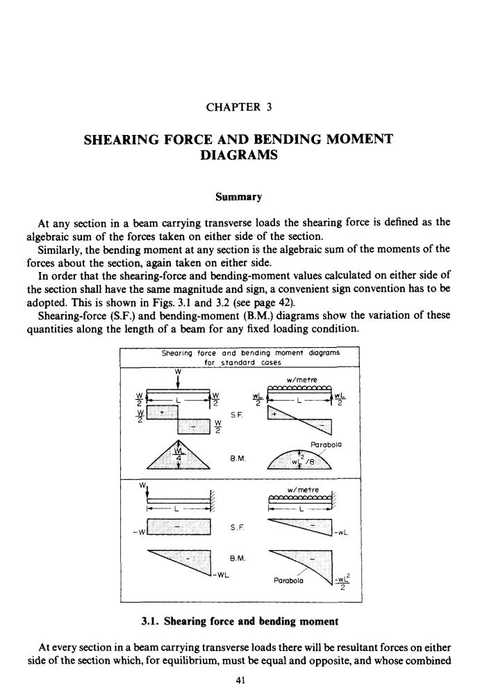
CHAPTER 3 SHEARING FORCE AND BENDING MOMENT DIAGRAMS Summary At any section in a beam carrying transverse loads the shearing force is defined as the algebraic sum of the forces taken on either side of the section. Similarly,the bending moment at any section is the algebraic sum of the moments of the forces about the section,again taken on either side. In order that the shearing-force and bending-moment values calculated on either side of the section shall have the same magnitude and sign,a convenient sign convention has to be adopted.This is shown in Figs.3.1 and 3.2 (see page 42). Shearing-force(S.F.)and bending-moment(B.M.)diagrams show the variation of these quantities along the length of a beam for any fixed loading condition. Shearing force and bending moment diagrams for standard cases w/metre xx S.F Parabola B.M. w生B w/metre sexxx S.F B.M. Parabola 3.1.Shearing force and bending moment At every section in a beam carrying transverse loads there will be resultant forces on either side of the section which,for equilibrium,must be equal and opposite,and whose combined 41
CHAPTER 3 SHEARING FORCE AND BENDING MOMENT DIAGRAMS Summary At any section in a beam carrying transverse loads the shearing force is defined as the algebraic sum of the forces taken on either side of the section. Similarly, the bending moment at any section is the algebraic sum of the moments of the forces about the section, again taken on either side. In order that the shearing-force and bending-moment values calculated on either side of the section shall have the same magnitude and sign, a convenient sign convention has to be adopted. This is shown in Figs. 3.1 and 3.2 (see page 42). Shearing-force (S.F.) and bending-moment (B.M.) diagrams show the variation of these quantities along the length of a beam for any fixed loading condition. Para bola BM I w. -wL SF I -w BM -Wf -WL - 2 3.1. Shearing force and bending moment At every section in a beam carrying transverse loads there will be resultant forces on either side of the section which, for equilibrium, must be equal and opposite, and whose combined 41
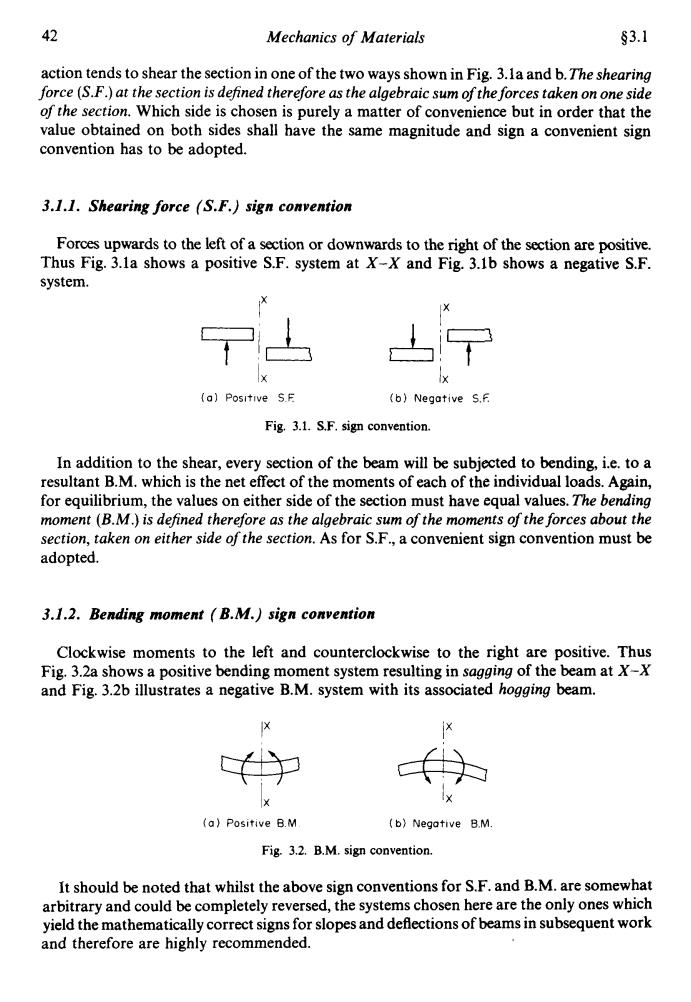
42 Mechanics of Materials §3.1 action tends to shear the section in one of the two ways shown in Fig.3.la and b.The shearing force (S.F.)at the section is defined therefore as the algebraic sum of the forces taken on one side of the section.Which side is chosen is purely a matter of convenience but in order that the value obtained on both sides shall have the same magnitude and sign a convenient sign convention has to be adopted. 3.1.1.Shearing force (S.F.)sign convention Forces upwards to the left of a section or downwards to the right of the section are positive. Thus Fig.3.1a shows a positive S.F.system at X-X and Fig.3.1b shows a negative S.F. system. (o】Positive S.E (b)Negative S.F Fig.3.1.S.F.sign convention. In addition to the shear,every section of the beam will be subjected to bending,i.e.to a resultant B.M.which is the net effect of the moments of each of the individual loads.Again, for equilibrium,the values on either side of the section must have equal values.The bending moment(B.M.)is defined therefore as the algebraic sum of the moments of the forces about the section,taken on either side of the section.As for S.F.,a convenient sign convention must be adopted. 3.1.2.Bending moment B.M.)sign convention Clockwise moments to the left and counterclockwise to the right are positive.Thus Fig.3.2a shows a positive bending moment system resulting in sagging of the beam at X-X and Fig.3.2b illustrates a negative B.M.system with its associated hogging beam. (a)Positive B.M (b)Negative B.M. Fig.3.2.B.M.sign convention. It should be noted that whilst the above sign conventions for S.F.and B.M.are somewhat arbitrary and could be completely reversed,the systems chosen here are the only ones which yield the mathematically correct signs for slopes and deflections of beams in subsequent work and therefore are highly recommended
42 Mechanics of Materials $3.1 action tends to shear the section in one of the two ways shown in Fig. 3.la and b. The shearing force (S.F.) at the section is defined therefore as the algebraic sum of the forces taken on one side of the section. Which side is chosen is purely a matter of convenience but in order that the value obtained on both sides shall have the same magnitude and sign a convenient sign convention has to be adopted. 3.1.1. Shearing force (S.F.) sign convention Forces upwards to the left of a section or downwards to the right of the section are positive. Thus Fig. 3.la shows a positive S.F. system at X-X and Fig. 3.lb shows a negative S.F. system. tX A!'? 723 (b) Negative Ix 5.E IX (a) Positive 5 F: Fig. 3.1. S.F. sign convention. In addition to the shear, every section of the beam will be subjected to bending, i.e. to a resultant B.M. which is the net effect of the moments of each of the individual loads. Again, for equilibrium, the values on either side of the section must have equal values. The bending moment (B.M.) is defined therefore as the algebraic sum of the moments of the forces about the section, taken on either side of the section. As for S.F., a convenient sign convention must be adopted. 3.1.2. Bending moment (B.M.) sign convention Clockwise moments to the left and counterclockwise to the right are positive. Thus Fig. 3.h shows a positive bending moment system resulting in sagging of the beam at X-X and Fig. 3.2b illustrates a negative B.M. system with its associated hogging beam. IX IX Wb IX e IX (a) Positive B M (b) Negative B.M Fig. 3.2. B.M. sign convention. It should be noted that whilst the above sign conventions for S.F. and B.M. are somewhat arbitrary and could be completely reversed, the systems chosen here are the only ones which yield the mathematically correct signs for slopes and deflections of beams in subsequent work and therefore are highly recommended
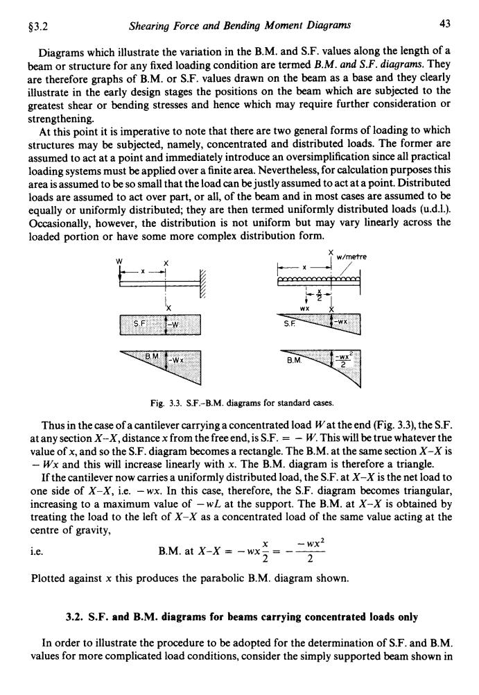
§3.2 Shearing Force and Bending Moment Diagrams 43 Diagrams which illustrate the variation in the B.M.and S.F.values along the length of a beam or structure for any fixed loading condition are termed B.M.and S.F.diagrams.They are therefore graphs of B.M.or S.F.values drawn on the beam as a base and they clearly illustrate in the early design stages the positions on the beam which are subjected to the greatest shear or bending stresses and hence which may require further consideration or strengthening. At this point it is imperative to note that there are two general forms of loading to which structures may be subjected,namely,concentrated and distributed loads.The former are assumed to act at a point and immediately introduce an oversimplification since all practical loading systems must be applied over a finite area.Nevertheless,for calculation purposes this area is assumed to be so small that the load can be justly assumed to act at a point.Distributed loads are assumed to act over part,or all,of the beam and in most cases are assumed to be equally or uniformly distributed;they are then termed uniformly distributed loads(u.d.1.). Occasionally,however,the distribution is not uniform but may vary linearly across the loaded portion or have some more complex distribution form. w/metre aaaaaaach0 S.F B.M Fig.3.3.S.F.-B.M.diagrams for standard cases. Thus in the case of a cantilever carrying a concentrated load Wat the end(Fig.3.3),the S.F. at any section X-X,distance x from the freeend,is S.F.=-W.This will be true whatever the value of x,and so the S.F.diagram becomes a rectangle.The B.M.at the same section X-X is -Wx and this will increase linearly with x.The B.M.diagram is therefore a triangle. If the cantilever now carries a uniformly distributed load,the S.F.at X-X is the net load to one side of X-X,i.e.-wx.In this case,therefore,the S.F.diagram becomes triangular, increasing to a maximum value of-wL at the support.The B.M.at X-X is obtained by treating the load to the left of X-X as a concentrated load of the same value acting at the centre of gravity, i.e. .-wx2 B.M.at X-X -wx2=-- 2 Plotted against x this produces the parabolic B.M.diagram shown. 3.2.S.F.and B.M.diagrams for beams carrying concentrated loads only In order to illustrate the procedure to be adopted for the determination of S.F.and B.M. values for more complicated load conditions,consider the simply supported beam shown in
$3.2 Shearing Force and Bending Moment Diagrams 43 Diagrams which illustrate the variation in the B.M. and S.F. values along the length of a beam or structure for any fixed loading condition are termed B.M. and S.F. diagrams. They are therefore graphs of B.M. or S.F. values drawn on the beam as a base and they clearly illustrate in the early design stages the positions on the beam which are subjected to the greatest shear or bending stresses and hence which may require further consideration or strengthening. At this point it is imperative to note that there are two general forms of loading to which structures may be subjected, namely, concentrated and distributed loads. The former are assumed to act at a point and immediately introduce an oversimplification since all practical loading systems must be applied over a finite area. Nevertheless, for calculation purposes this area is assumed to be so small that the load can be justly assumed to act at a point. Distributed loads are assumed to act over part, or all, of the beam and in most cases are assumed to be equally or uniformly distributed; they are then termed uniformly distributed loads (u.d.1.). Occasionally, however, the distribution is not uniform but may vary linearly across the loaded portion or have some more complex distribution form. 'X wx k Fig. 3.3. S.F.-B.M. diagrams for standard cases. Thus in the case of a cantilever carrying a concentrated load Wat the end (Fig. 3.3), the S.F. at any section X-X, distance x from the free end, is S.F. = - W. This will be true whatever the value of x, and so the S.F. diagram becomes a rectangle. The B.M. at the same section X-X is - Wx and this will increase linearly with x. The B.M. diagram is therefore a triangle. If the cantilever now carries a uniformly distributed load, the S.F. at X-X is the net load to one side of X-X, i.e. -wx. In this case, therefore, the S.F. diagram becomes triangular, increasing to a maximum value of - WL at the support. The B.M. at X-X is obtained by treating the load to the left of X-X as a concentrated load of the same value acting at the centre of gravity, i.e. X - wx2 B.M. at X-X = - wx - = - __ 2 2 Plotted against x this produces the parabolic B.M. diagram shown. 3.2. S.F. and B.M. diagrams for beams carrying concentrated loads only In order to illustrate the procedure to be adopted for the determination of S.F. and B.M. values for more complicated load conditions, consider the simply supported beam shown in
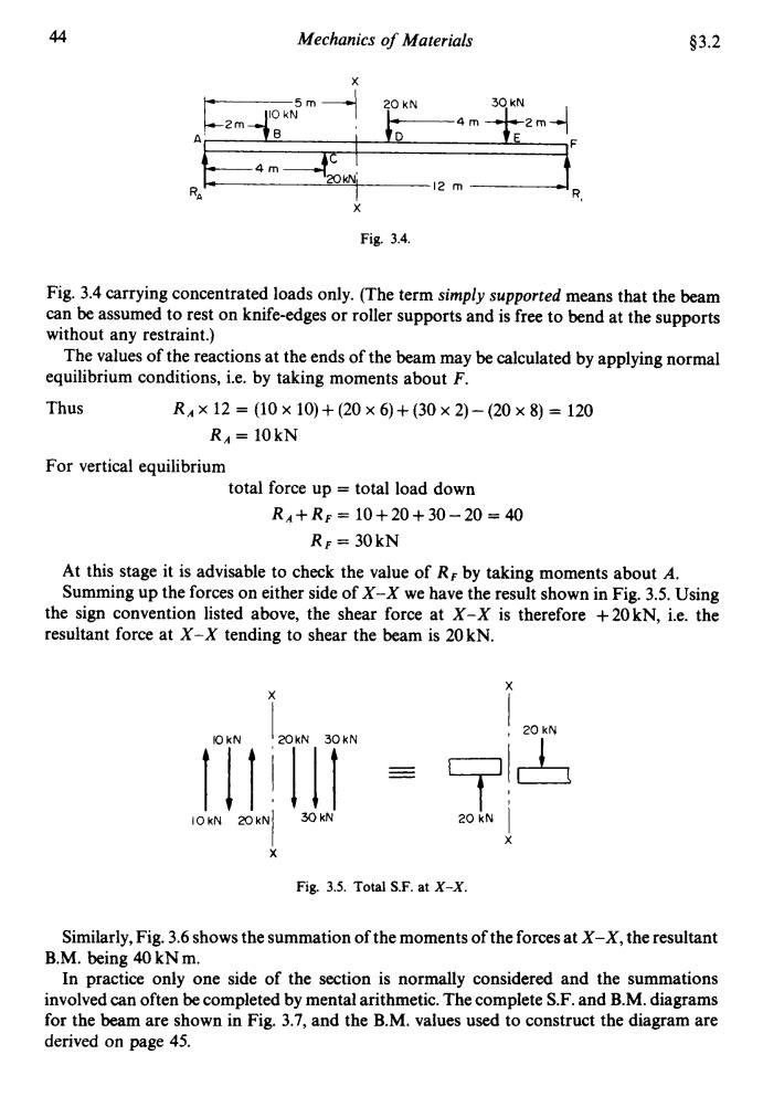
44 Mechanics of Materials §3.2 5m 20 kN 30 kN UIO kN -2m。 m 4 m R 12m Fig.3.4. Fig.3.4 carrying concentrated loads only.(The term simply supported means that the beam can be assumed to rest on knife-edges or roller supports and is free to bend at the supports without any restraint.) The values of the reactions at the ends of the beam may be calculated by applying normal equilibrium conditions,ie.by taking moments about F. Thus R4×12=(10×10)+(20×6)+(30×2)-(20×8)=120 R=10kN For vertical equilibrium total force up total load down R4+RF=10+20+30-20=40 R=30kN At this stage it is advisable to check the value of Rr by taking moments about A. Summing up the forces on either side of X-X we have the result shown in Fig.3.5.Using the sign convention listed above,the shear force at X-X is therefore +20kN,i.e.the resultant force at X-X tending to shear the beam is 20kN. 20 kN kN 20kN 30kN 30 kN 20 kN Fig.3.5.Total S.F.at X-X. Similarly,Fig.3.6 shows the summation of the moments of the forces at X-X,the resultant B.M.being 40 kN m. In practice only one side of the section is normally considered and the summations involved can often be completed by mental arithmetic.The complete S.F.and B.M.diagrams for the beam are shown in Fig.3.7,and the B.M.values used to construct the diagram are derived on page 45
44 Mechanics of Materials $3.2 Fig. 3.4. Fig. 3.4 carrying concentrated loads only. (The term simply supported means that the beam can be assumed to rest on knife-edges or roller supports and is free to bend at the supports without any restraint.) The values of the reactions at the ends of the beam may be calculated by applying normal equilibrium conditions, i.e. by taking moments about F. Thus RA x 12 = (10 x 10) + (20 x 6) + (30 x 2) - (20 x 8) = 120 RA = 10 kN For vertical equilibrium total force up = total load down RA+RF = 10+20+30-20 = 40 RF= 3OkN At this stage it is advisable to check the value of RF by taking moments about A. Summing up the forces on either side of X-X we have the result shown in Fig. 3.5. Using the sign convention listed above, the shear force at X-X is therefore +20kN, Le. the resultant force at X-X tending to shear the beam is 20 kN. IO 1* kN X I N ImkN 30kN 1~111 x)kN/ X 30kN i I , 20kN 20kN I Fig. 3.5. Total S.F. at X-X. X Similarly, Fig. 3.6 shows the summation of the moments of the forces at X-X, the resultant B.M. being 40 kNm. In practice only one side of the section is normally considered and the summations involved can often be completed by mental arithmetic. The complete S.F. and B.M. diagrams for the beam are shown in Fig. 3.7, and the B.M. values used to construct the diagram are derived on page 45

$3.2 Shearing Force and Bending Moment Diagrams 45 0x3 20x Rx7-210 40 kN m 40kN m Rx5=5020x,30x5 x Fig.3.6.Total B.M.at X-X. B.M.at A =0 B.M.atB=+(10×2) =+20kNm B.M.atC=+(10×4)-(10×2) =+20kNm B.M.atD=+(10×6)+(20×2)-(10×4)=+60kNm B.M.atE=+(30×2) =+60kNm B.M.at F =0 All the above values have been calculated from the moments of the forces to the left of each section considered except for E where forces to the right of the section are taken. IO kN 20kN 30 kN 10kN 30 kN 20 kN S.F diagram (kN) 20 10 -30 60 B.M.diagram (kN m) 20 Fig.3.7. It may be observed at this stage that the S.F.diagram can be obtained very quickly when working from the left-hand side,since after plotting the S.F.value at the support all subsequent steps are in the direction of and equal in magnitude to the applied loads,e.g. 10kN up at A,down 10kN at B,up 20kN at C,etc.,with horizontal lines joining the steps to show that the S.F.remains constant between points of application of concentrated loads. The S.F.and B.M.values at the left-hand support are determined by considering a section an infinitely small distance to the right of the support.The only load to the left (and hence the
$3.2 Shearing Force and Bending Moment Diagrams 45 R,x5=50 20x1, 30x5 I Ix 'X Fig. 3.6. Total B.M. at X-X. B.M. at A =o B.M. at B = + (10 x 2) = +20kNm B.M.atC= +(lOx4)-(1Ox2) = +20kNm B.M. at D = +(lox 6)+ (20 x 2)- (10 x 4) = +60kNm B.M. at E = + (30 x 2) = +60kNm B.M. at F =o All the above values have been calculated from the moments of the forces to the left of each section considered except for E where forces to the right of the section are taken. 10 Fig. 3.1. It may be observed at this stage that the S.F. diagram can be obtained very quickly when working from the left-hand side, since after plotting the S.F. value at the support all subsequent steps are in the direction of and equal in magnitude to the applied loads, e.g. 10 kN up at A, down 10 kN at B, up 20 kN at C, etc., with horizontal lines joining the steps to show that the S.F. remains constant between points of application of concentrated loads. The S.F. and B.M. values at the left-hand support are determined by considering a section an infinitely small distance to the right of the support. The only load to the left (and hence the