Parallel Prefix Sum(Scan)with CUDA and returns the array [,m,(⊕a,(a⊕4⊕..⊕an2l Example:If is addition,then the exclusive scan operation on the array [31704163, returns [0341111141622 An exclusive scan can be generated from an inclusive scan by shifting the resulting array right by one element and inserting the identity.Likewise,an inclusive scan can be generated from an exclusive scan by shifting the resulting array left,and inserting at the end the sum of the last element of the scan and the last element of the input array [1].For the remainder of this paper we will focus on the implementation of exclusive scan and refer to it simply as scan unless otherwise specified. Sequential Scan Implementing a sequential version of scan(that could be run in a single thread on a CPU,for example)is trivial.We simply loop over all the elements in the input array and add the value of the previous element of the input array to the sum computed for the previous element of the output array,and write the sum to the current element of the output array. void scan(float*output,float*input,int length) output[0]=0;//since this is a prescan,not a scan for(int j=1;j<length;++j) output[j]input[j-1]output[j-1]; This code performs exactly nadds for an array of length m,this is the minimum number of adds required to produce the scanned array.When we develop our parallel version of scan, we would like it to be work-efficient.This means do no more addition operations (or work) than the sequential version.In other words the two implementations should have the same work complexcity,O(n). A Naive Parallel Scan for d:=I to logan do d:=0 to logn-1 forall kin parallel do k=0n-1 if kz 2d then=x+ 2^d Algorithm 1:A sum scan algorithm that is not work-efficient. April 2007
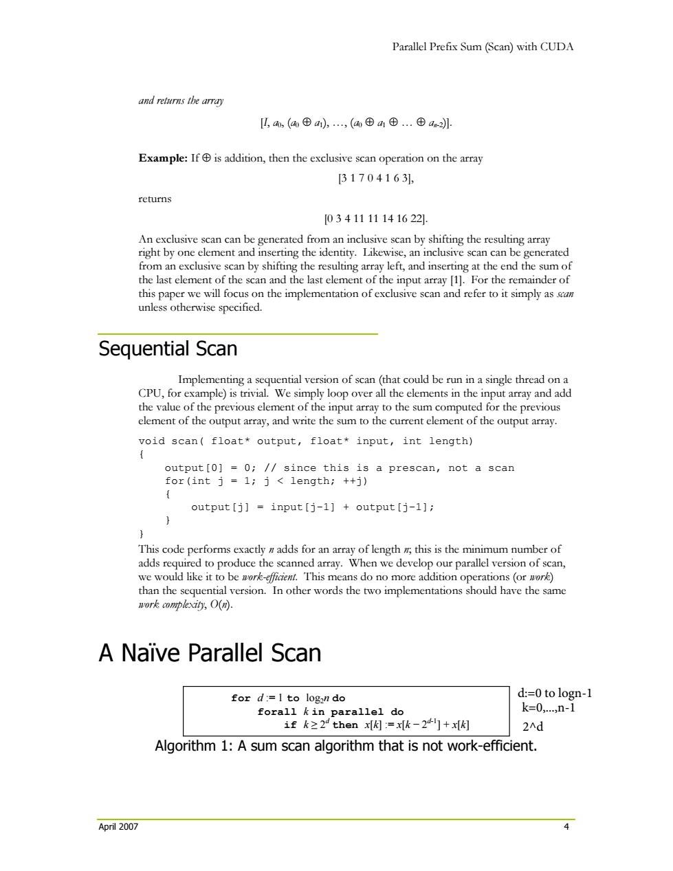
Parallel Prefix Sum (Scan) with CUDA April 2007 4 and returns the array [I, a0, (a0 ⊕ a1), …, (a0 ⊕ a1 ⊕ … ⊕ an-2)]. Example: If ⊕ is addition, then the exclusive scan operation on the array [3 1 7 0 4 1 6 3], returns [0 3 4 11 11 14 16 22]. An exclusive scan can be generated from an inclusive scan by shifting the resulting array right by one element and inserting the identity. Likewise, an inclusive scan can be generated from an exclusive scan by shifting the resulting array left, and inserting at the end the sum of the last element of the scan and the last element of the input array [1]. For the remainder of this paper we will focus on the implementation of exclusive scan and refer to it simply as scan unless otherwise specified. Sequential Scan Implementing a sequential version of scan (that could be run in a single thread on a CPU, for example) is trivial. We simply loop over all the elements in the input array and add the value of the previous element of the input array to the sum computed for the previous element of the output array, and write the sum to the current element of the output array. void scan( float* output, float* input, int length) { output[0] = 0; // since this is a prescan, not a scan for(int j = 1; j < length; ++j) { output[j] = input[j-1] + output[j-1]; } } This code performs exactly n adds for an array of length n; this is the minimum number of adds required to produce the scanned array. When we develop our parallel version of scan, we would like it to be work-efficient. This means do no more addition operations (or work) than the sequential version. In other words the two implementations should have the same work complexity, O(n). A Naïve Parallel Scan Algorithm 1: A sum scan algorithm that is not work-efficient. for d := 1 to log2n do forall k in parallel do if k ≥ 2d then x[k] := x[k − 2d-1] + x[k] k=0,...,n-1 d:=0 to logn-1 2^d
Parallel Prefix Sum(Scan)with CUDA The pseudocode in Algorithm 1 shows a naive parallel scan implementation.This algorithm is based on the scan algorithm presented by Hillis and Steele![4],and demonstrated for GPUs by Horn [5].The problem with Algorithm 1 is apparent if we examine its work complexity.The rtm performs)ddtion operations. Remember that a sequential scan performs O()adds.Therefore,this naive implementation is not work-efficient.The factor of log2 n can have a large effect on performance.In the case of a scan of 1 million elements,the performance difference between this naive implementation and a theoretical work-efficient parallel implementation would be almost a factor of 20. Algorithm 1 assumes that there are as many processors as data elements.On a GPU running CUDA,this is not usually the case.Instead,the forall is automatically divided into small parallel batches(called warp)that are executed sequentially on a multiprocessor. A G80 GPU executes warps of 32 threads in parallel.Because not all threads run simultaneously for arrays larger than the warp size,the algorithm above will not work because it performs the scan in place on the array.The results of one warp will be overwritten by threads in another warp. To solve this problem,we need to double-buffer the array we are scanning.We use two temporary arrays(temp[2][n])to do this.Pseudocode for this is given in Algorithm 2, and CUDA C code for the naive scan is given in Listing 1.Note that this code will run on only a single thread block of the GPU,and so the size of the arrays it can process is limited (to 512 elements on G80 GPUs).Extension of scan to large arrays is discussed later. for d:=1 to logan do d:=0 to logn-1 forall kin parallel do ifk≥24then x[oud[附:=x[imk-24]+x[im[ 2^d else x[out:=x[in]k闷 swap (in,out) Algorithm 2:A double-buffered version of the sum scan from Algorithm 1. 1 Note that while we call this a naire scan in the context of CUDA and NVIDIA GPUs,it was not necessarily naive for a Connection Machine 3],which is the machine Hillis and Steele were focused on.Related to work complexity is the concept of step complexiny,which is the number of steps that the algorithm executes.The Connection Machine was a SIMD machine with many thousands of processors.In the limit where the number of processors equals the number of elements to be scanned,execution time is dominated by step complexity rather than work complexity.Algorithm 1 has a step complexity of o(log compared to the O()step complexity of the sequential algorithm, and is therefore step efficient. April 2007 5
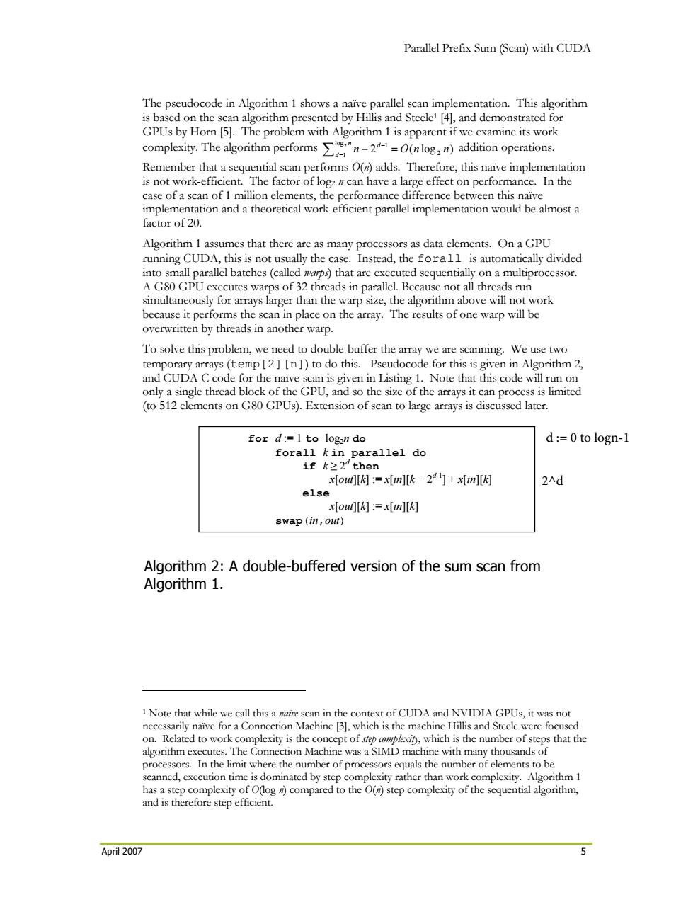
Parallel Prefix Sum (Scan) with CUDA April 2007 5 The pseudocode in Algorithm 1 shows a naïve parallel scan implementation. This algorithm is based on the scan algorithm presented by Hillis and Steele1 [4], and demonstrated for GPUs by Horn [5]. The problem with Algorithm 1 is apparent if we examine its work complexity. The algorithm performs )log(2 2 log 1 2 1 nnOnn d d ∑ =− = − addition operations. Remember that a sequential scan performs O(n) adds. Therefore, this naïve implementation is not work-efficient. The factor of log2 n can have a large effect on performance. In the case of a scan of 1 million elements, the performance difference between this naïve implementation and a theoretical work-efficient parallel implementation would be almost a factor of 20. Algorithm 1 assumes that there are as many processors as data elements. On a GPU running CUDA, this is not usually the case. Instead, the forall is automatically divided into small parallel batches (called warps) that are executed sequentially on a multiprocessor. A G80 GPU executes warps of 32 threads in parallel. Because not all threads run simultaneously for arrays larger than the warp size, the algorithm above will not work because it performs the scan in place on the array. The results of one warp will be overwritten by threads in another warp. To solve this problem, we need to double-buffer the array we are scanning. We use two temporary arrays (temp[2][n]) to do this. Pseudocode for this is given in Algorithm 2, and CUDA C code for the naïve scan is given in Listing 1. Note that this code will run on only a single thread block of the GPU, and so the size of the arrays it can process is limited (to 512 elements on G80 GPUs). Extension of scan to large arrays is discussed later. Algorithm 2: A double-buffered version of the sum scan from Algorithm 1. 1 Note that while we call this a naïve scan in the context of CUDA and NVIDIA GPUs, it was not necessarily naïve for a Connection Machine [3], which is the machine Hillis and Steele were focused on. Related to work complexity is the concept of step complexity, which is the number of steps that the algorithm executes. The Connection Machine was a SIMD machine with many thousands of processors. In the limit where the number of processors equals the number of elements to be scanned, execution time is dominated by step complexity rather than work complexity. Algorithm 1 has a step complexity of O(log n) compared to the O(n) step complexity of the sequential algorithm, and is therefore step efficient. for d := 1 to log2n do forall k in parallel do if k ≥ 2d then x[out][k] := x[in][k − 2d-1] + x[in][k] else x[out][k] := x[in][k] swap(in,out) d := 0 to logn-1 2^d