Experiment 6 Investigation of the properties of Magnetic Material Magnetic material has been widely used in electric power,communication,electronic machine, autocar,computer,information storage and so on.Its two basic features can be shown by magnetic hysteresis loop and Curie temperature.The former one reflects the magnetization character of magnetic material in magnetic field,and the later one is related to the phase transition from ferromagnetic state to paramagnetic state. In this experiment,the Curie temperature and dynamic hysteresis loop of soft ferromagnetic material will be measured. 【Aim of the experiment】. 1. Get the knowledge of magnetic hysteresis loop,magnetization curve and Curie temperature.Have a deep understanding of some concepts about ferromagnetic material,such as coercive force,residual magnetic flux density,saturated magnetic flux density and magnetic permeability. 2. Observe hysteresis loop through an oscilloscope. Measure the Curie temperature of the ferromagnetic material given in this experiment. 【Principle of the experiment】. 1.The magnetization properties Magnetism is a property of materials that respond to an applied magnetic field.The rule of magnetization can be described by magnetic flux density (magnetic induction)B, B◆I A B-H M-H H T Fig.1 Magnetization curve of ferromagnet and L-H curve Fig.2 L-T curve of ferromagnet
- - 1 Experiment 6 Investigation of the properties of Magnetic Material Magnetic material has been widely used in electric power, communication, electronic machine, autocar, computer, information storage and so on. Its two basic features can be shown by magnetic hysteresis loop and Curie temperature. The former one reflects the magnetization character of magnetic material in magnetic field, and the later one is related to the phase transition from ferromagnetic state to paramagnetic state. In this experiment, the Curie temperature and dynamic hysteresis loop of soft ferromagnetic material will be measured. 【Aim of the experiment】 1. Get the knowledge of magnetic hysteresis loop, magnetization curve and Curie temperature. Have a deep understanding of some concepts about ferromagnetic material, such as coercive force, residual magnetic flux density, saturated magnetic flux density and magnetic permeability. 2. Observe hysteresis loop through an oscilloscope. 3. Measure the Curie temperature of the ferromagnetic material given in this experiment. 【Principle of the experiment】 1 .The magnetization properties Magnetism is a property of materials that respond to an applied magnetic field. The rule of magnetization can be described by magnetic flux density (magnetic induction) B, Fig. 1 Magnetization curve of ferromagnet and μ ~ H curve Fig. 2 μ ~ T curve of ferromagnet
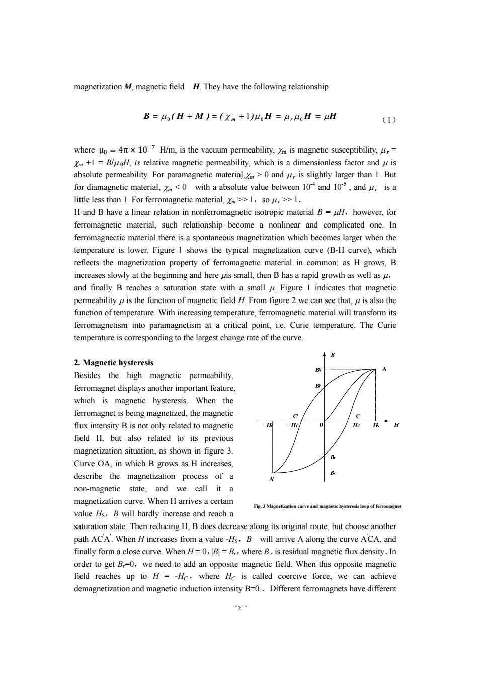
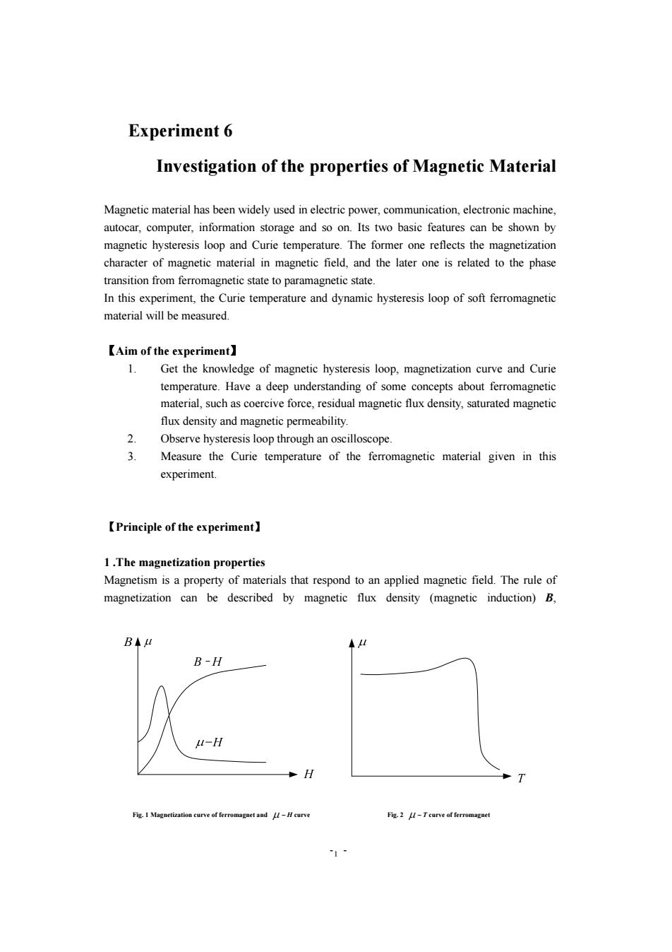
magnetization M,magnetic field H.They have the following relationship B=uo(H+M)=(m+1)uoH=u,oH=H (1) where o=4nx 10-7 H/m,is the vacuum permeability,m is magnetic susceptibility,r= m+1=BluoH,is relative magnetic permeability,which is a dimensionless factor and u is absolute permeability.For paramagnetic material,>0 and u is slightly larger than 1.But for diamagnetic material,m with a absolute value between 10 and 105,and is a little less than 1.For ferromagnetic material,>>1,so>>1. H and B have a linear relation in nonferromagnetic isotropic material B=uH,however,for ferromagnetic material,such relationship become a nonlinear and complicated one.In ferromagnectic material there is a spontaneous magnetization which becomes larger when the temperature is lower.Figure 1 shows the typical magnetization curve (B-H curve),which reflects the magnetization property of ferromagnetic material in common:as H grows,B increases slowly at the beginning and here tis small,then B has a rapid growth as well as 4, and finally B reaches a saturation state with a small 4.Figure 1 indicates that magnetic permeability u is the function of magnetic field H.From figure 2 we can see that,u is also the function of temperature.With increasing temperature,ferromagnetic material will transform its ferromagnetism into paramagnetism at a critical point,i.e.Curie temperature.The Curie temperature is corresponding to the largest change rate of the curve. 2.Magnetic hysteresis Besides the high magnetic permeability, ferromagnet displays another important feature, which is magnetic hysteresis.When the ferromagnet is being magnetized,the magnetic flux intensity B is not only related to magnetic He 0 field H,but also related to its previous magnetization situation,as shown in figure 3. Curve OA,in which B grows as H increases, describe the magnetization process of a non-magnetic state,and we call it a magnetization curve.When H arrives a certain Fig.3 Magnetization curve and magnetic hvsteresis loop of ferromagnet value Hs,B will hardly increase and reach a saturation state.Then reducing H,B does decrease along its original route,but choose another path ACA.When H increases from a value-Hs,B will arrive A along the curve A'CA,and finally form a close curve.When H=0,B=B,,where B,is residual magnetic flux density.In order to get B,-0,we need to add an opposite magnetic field.When this opposite magnetic field reaches up to H=-Hc,where Hc is called coercive force,we can achieve demagnetization and magnetic induction intensity B-0..Different ferromagnets have different 2
- - 2 magnetization M, magnetic field H. They have the following relationship B = μ 0 ( H + M ) = ( χ m + 1 )μ 0 H = μ r μ 0 H = μH (1) where µ ൌ 4π ൈ 10ି H/m, is the vacuum permeability, χm is magnetic susceptibility, μ r = χm +1 = B/μ 0H, is relative magnetic permeability, which is a dimensionless factor and μ is absolute permeability. For paramagnetic material,χm > 0 and μ r is slightly larger than 1. But for diamagnetic material, χm < 0 with a absolute value between 10-4 and 10-5 , and μ r is a little less than 1. For ferromagnetic material, χm >> 1,so μ r >> 1. H and B have a linear relation in nonferromagnetic isotropic material B = μH,however, for ferromagnetic material, such relationship become a nonlinear and complicated one. In ferromagnectic material there is a spontaneous magnetization which becomes larger when the temperature is lower. Figure 1 shows the typical magnetization curve (B-H curve), which reflects the magnetization property of ferromagnetic material in common: as H grows, B increases slowly at the beginning and here μis small, then B has a rapid growth as well as μ, and finally B reaches a saturation state with a small μ. Figure 1 indicates that magnetic permeability μ is the function of magnetic field H. From figure 2 we can see that, μ is also the function of temperature. With increasing temperature, ferromagnetic material will transform its ferromagnetism into paramagnetism at a critical point, i.e. Curie temperature. The Curie temperature is corresponding to the largest change rate of the curve. 2. Magnetic hysteresis Besides the high magnetic permeability, ferromagnet displays another important feature, which is magnetic hysteresis. When the ferromagnet is being magnetized, the magnetic flux intensity B is not only related to magnetic field H, but also related to its previous magnetization situation, as shown in figure 3. Curve OA, in which B grows as H increases, describe the magnetization process of a non-magnetic state, and we call it a magnetization curve. When H arrives a certain value HS,B will hardly increase and reach a saturation state. Then reducing H, B does decrease along its original route, but choose another path AC' A' . When H increases from a value -HS,B will arrive A along the curve A' CA, and finally form a close curve. When H = 0,|B| = Br,where B r is residual magnetic flux density.In order to get Br=0,we need to add an opposite magnetic field. When this opposite magnetic field reaches up to H = -HC , where HC is called coercive force, we can achieve demagnetization and magnetic induction intensity B=0..Different ferromagnets have different Fig. 3 Magnetization curve and magnetic hysteresis loop of ferromagnet
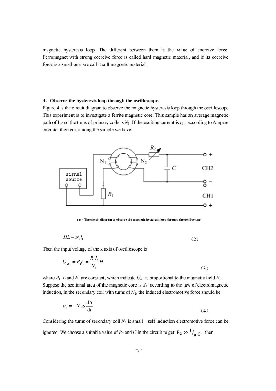
magnetic hysteresis loop.The different between them is the value of coercive force. Ferromagnet with strong coercive force is called hard magnetic material,and if its coercive force is a small one,we call it soft magnetic material. 3.Observe the hysteresis loop through the oscilloscope. Figure 4 is the circuit diagram to observe the magnetic hysteresis loop through the oscilloscope This experiment is to investigate a ferrite magnetic core.This sample has an average magnetic path of L and the turns of primary coils is Ni.If the exciting current is i,according to Ampere circuital theorem,among the sample we have 0+ CH2 signal source 8= R CHI 0+ Fig.4 The circuit diagram to observe the magnetic hysteresis loop through the oscilloscope HL=N i (2) Then the input voltage of the x axis of oscilloscope is U&,=Ri=- LH (3) where R,L and N are constant,which indicate URi is proportional to the magnetic field H. Suppose the sectional area of the magnetic core is S,according to the law of electromagnetic induction,in the secondary coil with turns of N2,the induced electromotive force should be E:=-N,s dB dt (4) Considering the turns of secondary coil N2 is small,self induction electromotive force can be ignored.We choose a suitable value of Rand Cin the circuit to get Rthen 3
- - 3 magnetic hysteresis loop. The different between them is the value of coercive force. Ferromagnet with strong coercive force is called hard magnetic material, and if its coercive force is a small one, we call it soft magnetic material. 3.Observe the hysteresis loop through the oscilloscope. Figure 4 is the circuit diagram to observe the magnetic hysteresis loop through the oscilloscope. This experiment is to investigate a ferrite magnetic core. This sample has an average magnetic path of L and the turns of primary coils is N1. If the exciting current is i1,according to Ampere circuital theorem, among the sample we have 1 1 HL = N i (2) Then the input voltage of the x axis of oscilloscope is H N R L U R i R 1 1 1 1 1 = = (3) where R1, L and N1 are constant, which indicate UR1 is proportional to the magnetic field H. Suppose the sectional area of the magnetic core is S,according to the law of electromagnetic induction, in the secondary coil with turns of N2, the induced electromotive force should be t B N S d d 2 = − 2 ε (4) Considering the turns of secondary coil N2 is small,self induction electromotive force can be ignored. We choose a suitable value of R2 and C in the circuit to get Rଶ ب 1 ωC ൗ ,then Fig. 4 The circuit diagram to observe the magnetic hysteresis loop through the oscilloscope
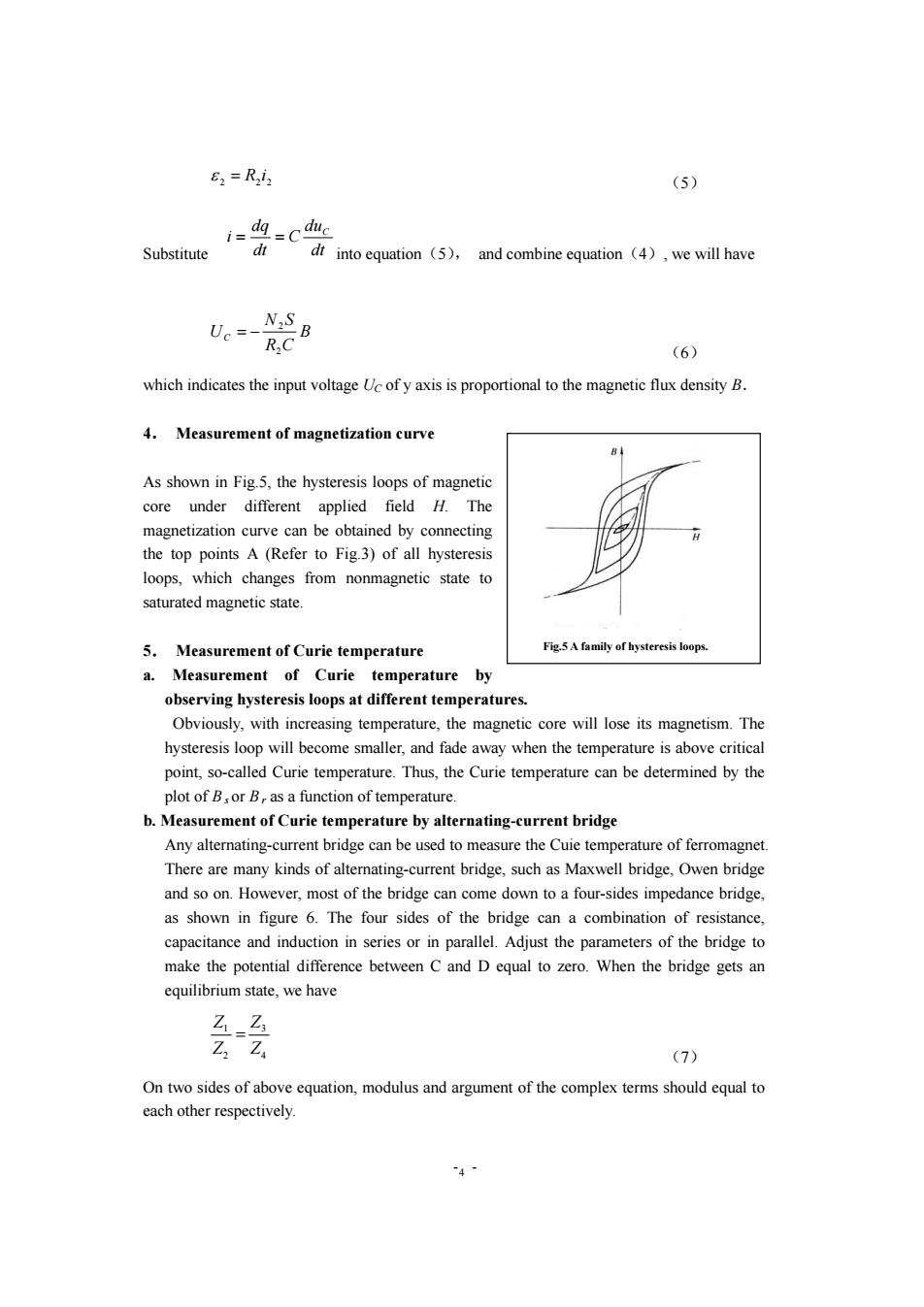
62=Ri3 (5) dg =Cduc is Substitute dt dt into equation (5),and combine equation (4),we will have Uc=- B R,C (6) which indicates the input voltage Uc ofy axis is proportional to the magnetic flux density B. 4.Measurement of magnetization curve As shown in Fig.5,the hysteresis loops of magnetic core under different applied field H.The magnetization curve can be obtained by connecting the top points A (Refer to Fig.3)of all hysteresis loops,which changes from nonmagnetic state to saturated magnetic state. 5.Measurement of Curie temperature Fig.5 A family of hysteresis loops. a.Measurement of Curie temperature by observing hysteresis loops at different temperatures. Obviously,with increasing temperature,the magnetic core will lose its magnetism.The hysteresis loop will become smaller,and fade away when the temperature is above critical point,so-called Curie temperature.Thus,the Curie temperature can be determined by the plot of B or B,as a function of temperature. b.Measurement of Curie temperature by alternating-current bridge Any alternating-current bridge can be used to measure the Cuie temperature of ferromagnet. There are many kinds of alternating-current bridge,such as Maxwell bridge,Owen bridge and so on.However,most of the bridge can come down to a four-sides impedance bridge, as shown in figure 6.The four sides of the bridge can a combination of resistance, capacitance and induction in series or in parallel.Adjust the parameters of the bridge to make the potential difference between C and D equal to zero.When the bridge gets an equilibrium state,we have 名-召 Z Z. (7) On two sides of above equation,modulus and argument of the complex terms should equal to each other respectively. ”4
- - 4 2 2 2 ε = R i (5) Substitute into equation(5), and combine equation(4), we will have B R C N S UC 2 2 = − (6) which indicates the input voltage UC of y axis is proportional to the magnetic flux density B. 4. Measurement of magnetization curve As shown in Fig.5, the hysteresis loops of magnetic core under different applied field H. The magnetization curve can be obtained by connecting the top points A (Refer to Fig.3) of all hysteresis loops, which changes from nonmagnetic state to saturated magnetic state. 5. Measurement of Curie temperature a. Measurement of Curie temperature by observing hysteresis loops at different temperatures. Obviously, with increasing temperature, the magnetic core will lose its magnetism. The hysteresis loop will become smaller, and fade away when the temperature is above critical point, so-called Curie temperature. Thus, the Curie temperature can be determined by the plot of B s or B r as a function of temperature. b. Measurement of Curie temperature by alternating-current bridge Any alternating-current bridge can be used to measure the Cuie temperature of ferromagnet. There are many kinds of alternating-current bridge, such as Maxwell bridge, Owen bridge and so on. However, most of the bridge can come down to a four-sides impedance bridge, as shown in figure 6. The four sides of the bridge can a combination of resistance, capacitance and induction in series or in parallel. Adjust the parameters of the bridge to make the potential difference between C and D equal to zero. When the bridge gets an equilibrium state, we have 4 3 2 1 Z Z Z Z = (7) On two sides of above equation, modulus and argument of the complex terms should equal to each other respectively. dt du C dt dq i C = = Fig.5 A family of hysteresis loops
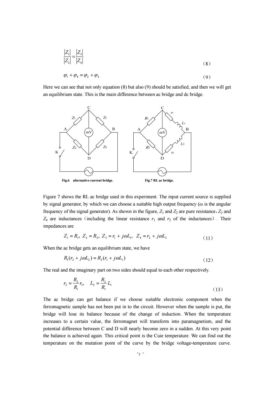
☑_z lzIz.l (8) p1+p4=p2+p3 (9) Here we can see that not only equation(8)but also(9)should be satisfied,and then we will get an equilibrium state.This is the main difference between ac bridge and de bridge. Z B mV R阳 D D Fig.6 alternative-current bridge. Fig.7 RL ac bridge. Figure 7 shows the RL ac bridge used in this experiment.The input current source is supplied by signal generator,by which we can choose a suitable high output frequency (is the angular frequency of the signal generator).As shown in the figure,Z and Z2 are pure resistance,Z3 and Z4 are inductances (including the linear resistance r and r2 of the inductances).Their impedances are Z,=R,Z2=R2,Z3=5+j0L,Z4=53+joL2 (11) When the ac bridge gets an equilibrium state,we have R(r2 joL)=R2(r+joL) (12) The real and the imaginary part on two sides should equal to each other respectively. 3= R R,L R (13) The ac bridge can get balance if we choose suitable electronic component when the ferromagnetic sample has not been put in to the circuit.However when the sample is put,the bridge will lose its balance because of the change of induction.When the temperature increases to a certain value,the ferromagnet will transform into paramagnetism,and the potential difference between C and D will nearly become zero in a sudden.At this very point the balance is achieved again.This critical point is the Cuie temperature.We can find out the temperature on the mutation point of the curve by the bridge voltage-temperature curve
- - 5 4 3 2 1 Z Z Z Z = (8) ϕ1 +ϕ 4 =ϕ 2 +ϕ3 (9) Here we can see that not only equation (8) but also (9) should be satisfied, and then we will get an equilibrium state. This is the main difference between ac bridge and dc bridge. Figure 7 shows the RL ac bridge used in this experiment. The input current source is supplied by signal generator, by which we can choose a suitable high output frequency (ω is the angular frequency of the signal generator). As shown in the figure, Z1 and Z2 are pure resistance,Z3 and Z4 are inductances(including the linear resistance r1 and r2 of the inductances). Their impedances are 1 1 2 2 3 1 1 4 2 2 Z = R, Z = R , Z = r + jωL, Z = r + jωL (11) When the ac bridge gets an equilibrium state, we have ( ) ( ) 1 2 2 2 1 L1 R r + jωL = R r + jω (12) The real and the imaginary part on two sides should equal to each other respectively. 1 1 2 1 2 1 2 2 L R R r L R R r = , = (13) The ac bridge can get balance if we choose suitable electronic component when the ferromagnetic sample has not been put in to the circuit. However when the sample is put, the bridge will lose its balance because of the change of induction. When the temperature increases to a certain value, the ferromagnet will transform into paramagnetism, and the potential difference between C and D will nearly become zero in a sudden. At this very point the balance is achieved again. This critical point is the Cuie temperature. We can find out the temperature on the mutation point of the curve by the bridge voltage-temperature curve. Fig.6 alternative-current bridge. Fig.7 RL ac bridge