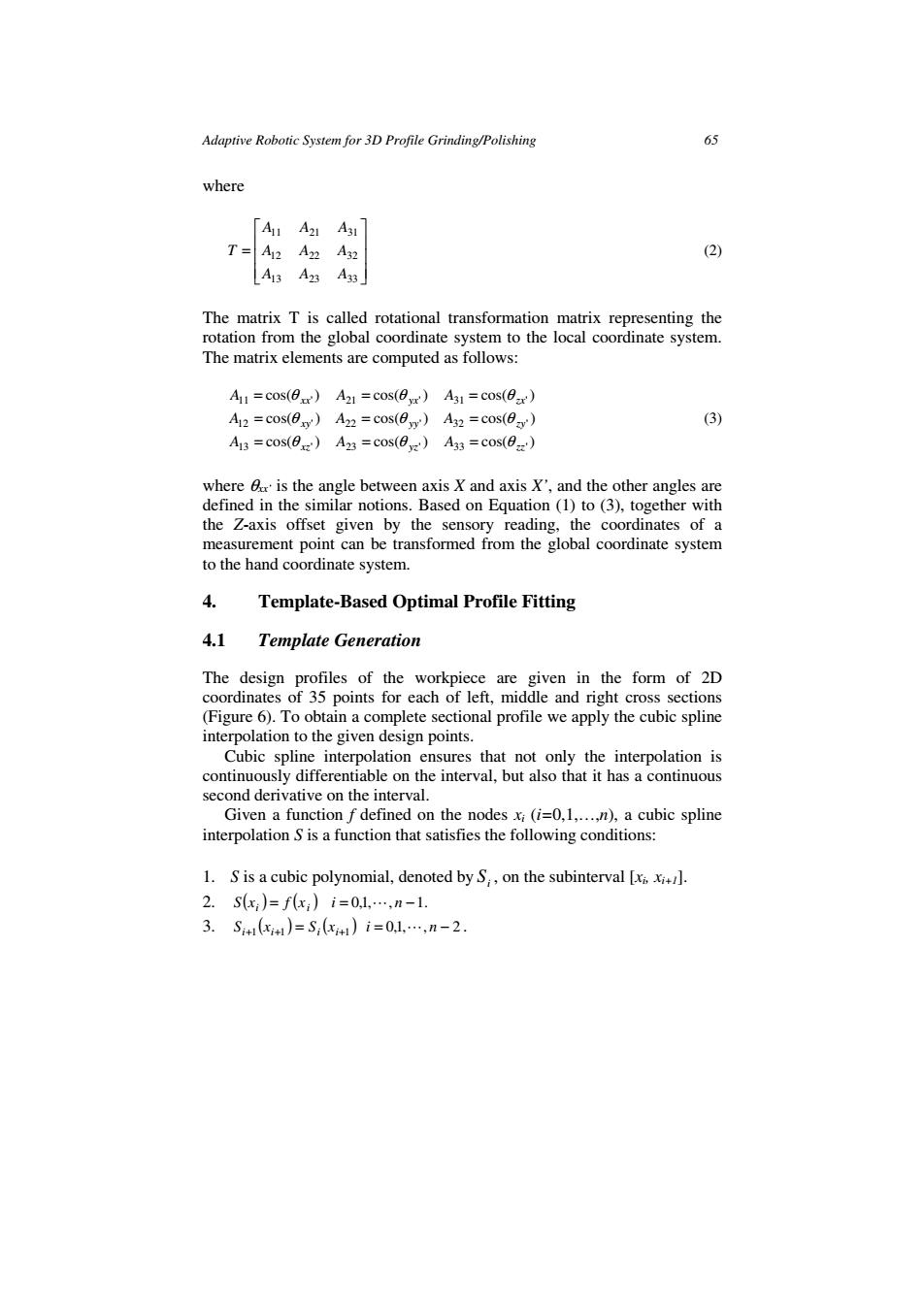
Adaptive Robotic System for 3D Profile Grinding/Polishing 65 where 「A11A21 A31 T=A12 A2 A32 (2) A13A23A33 The matrix T is called rotational transformation matrix representing the rotation from the global coordinate system to the local coordinate system. The matrix elements are computed as follows: A11=cos()A21 =cos(vr)A31=cos() A12 =cos(ey)A22 =cos(ey)A32 =cos(ev) (3) A13=cos(0z)A23=c0s(8z)A33=c0s(8x) where is the angle between axis X and axis X',and the other angles are defined in the similar notions.Based on Equation (1)to(3),together with the Z-axis offset given by the sensory reading,the coordinates of a measurement point can be transformed from the global coordinate system to the hand coordinate system. 4. Template-Based Optimal Profile Fitting 4.1 Template Generation The design profiles of the workpiece are given in the form of 2D coordinates of 35 points for each of left,middle and right cross sections (Figure 6).To obtain a complete sectional profile we apply the cubic spline interpolation to the given design points. Cubic spline interpolation ensures that not only the interpolation is continuously differentiable on the interval,but also that it has a continuous second derivative on the interval. Given a function f defined on the nodes xi(i=0,1,...,n),a cubic spline interpolation S is a function that satisfies the following conditions: 1.S is a cubic polynomial,denoted by S,,on the subinterval [xixi+l. 2.Sx;)=fx;)i=0,l,…,n-1. 3.Si+1(1)=S,(x#1)i=0l,…,n-2
Adaptive Robotic System for 3D Profile Grinding/Polishing 65 where = 13 23 33 12 22 32 11 21 31 A A A A A A A A A T (2) The matrix T is called rotational transformation matrix representing the rotation from the global coordinate system to the local coordinate system. The matrix elements are computed as follows: cos( ) cos( ) cos( ) cos( ) cos( ) cos( ) cos( ) cos( ) cos( ) 13 ' 23 ' 33 ' 12 ' 22 ' 32 ' 11 ' 21 ' 31 ' xz yz zz xy yy zy xx yx zx A A A A A A A A A θ θ θ θ θ θ θ θ θ = = = = = = = = = (3) where θxx’ is the angle between axis X and axis X’, and the other angles are defined in the similar notions. Based on Equation (1) to (3), together with the Z-axis offset given by the sensory reading, the coordinates of a measurement point can be transformed from the global coordinate system to the hand coordinate system. 4. Template-Based Optimal Profile Fitting 4.1 Template Generation The design profiles of the workpiece are given in the form of 2D coordinates of 35 points for each of left, middle and right cross sections (Figure 6). To obtain a complete sectional profile we apply the cubic spline interpolation to the given design points. Cubic spline interpolation ensures that not only the interpolation is continuously differentiable on the interval, but also that it has a continuous second derivative on the interval. Given a function f defined on the nodes xi (i=0,1,…,n), a cubic spline interpolation S is a function that satisfies the following conditions: 1. S is a cubic polynomial, denoted by i S , on the subinterval [xi, xi+1]. 2. ( ) ( ) i i xS = xf i = L,,1,0 n − .1 3. ( ) ( ) i+1 i+1 = ii +1 S x S x i = L,,1,0 n − 2

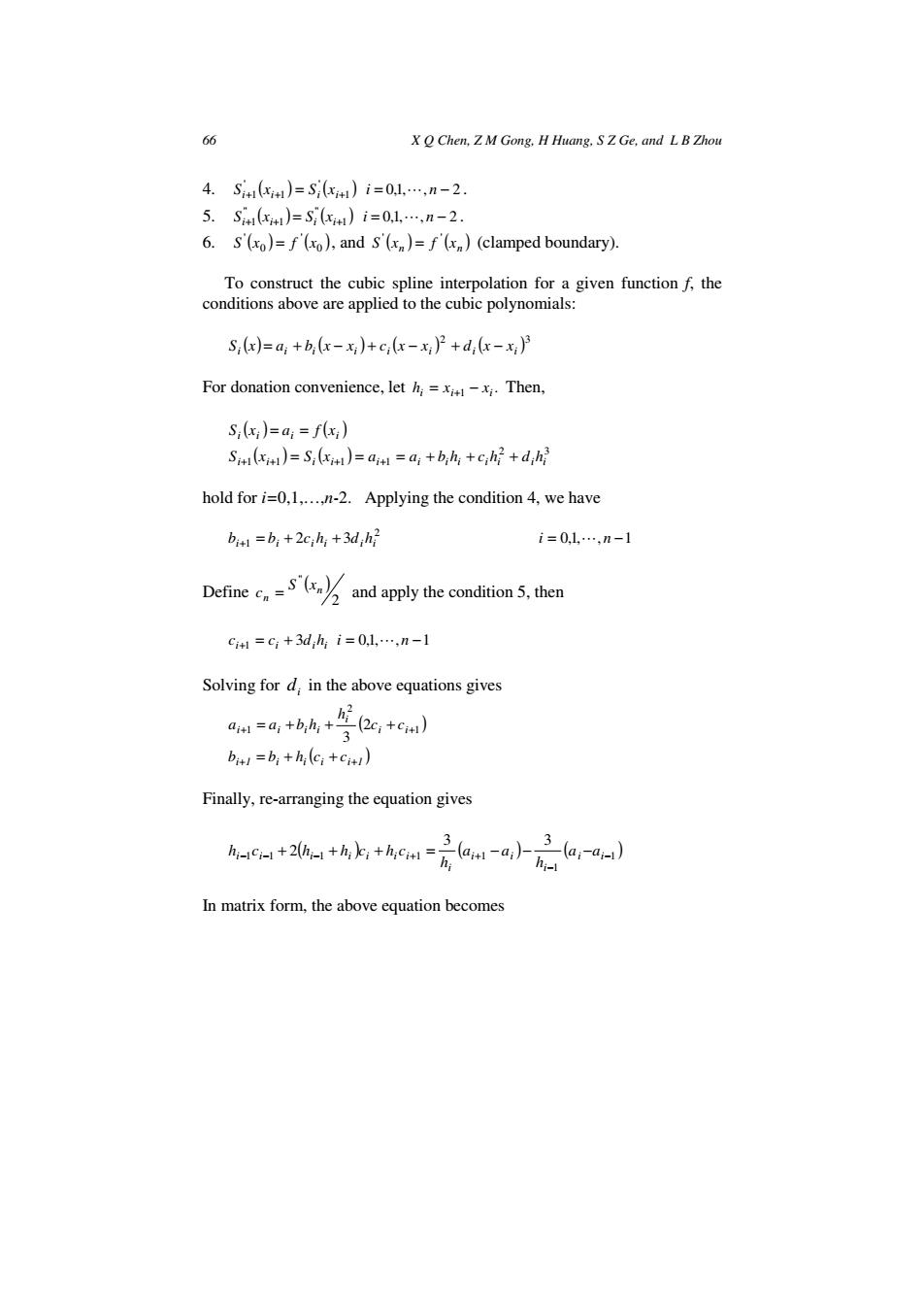
66 X Q Chen,Z M Gong.H Huang.SZ Ge,and L B Zhou 4.Si1(k1)=Sc)i=0.l,…,n-2. 5.Si(xt1)=S(x1)i=0,1,…,n-2. 6.S(xo)=f'(xo),and S')=f)(clamped boundary). To construct the cubic spline interpolation for a given function f,the conditions above are applied to the cubic polynomials: S;(x)=a;+b(x-x)+cx-x)2+di(x-x) For donation convenience,leth;=x-x.Then, S;(xi)=a;=f(xi) Si)=S;i)=aim=ai+bh+ch2+dhi hold for i=0,1,...,n-2.Applying the condition 4,we have bitt =bi+2cih +3d h2 i=0,l…,n-1 Defineand apply the condition 5,then ci1=C+3d,hi=0l,…,n-1 Solving for d in the above equations gives a=a,+hh+bc,+c) 3 bitl =bi+hi(ci+cit!) Finally,re-arranging the equation gives m=(ar In matrix form,the above equation becomes
66 X Q Chen, Z M Gong, H Huang, S Z Ge, and L B Zhou 4. ( ) ( ) 1 ' 1 ' i+1 i+ = ii + S x S x i = L,,1,0 n − 2 . 5. ( ) ( ) 1 " 1 " i+1 i+ = ii + S x S x i = L,,1,0 n − 2 . 6. ( ) ( ) 0 ' 0 ' S x = xf , and ( ) ( ) n n S x xf ' ' = (clamped boundary). To construct the cubic spline interpolation for a given function f, the conditions above are applied to the cubic polynomials: ( ) ( ) ( ) ( ) 2 3 i i i i i i i i S x = a + b x − x + c x − x + d x − x For donation convenience, let . i i 1 i h = x − x + Then, ( ) ( ) ii i i S x = a = xf ( ) ( ) 2 3 i 1 i 1 ii 1 i 1 i ii ii ii S x = S x = a = a + hb + hc + hd + + + + hold for i=0,1,…,n-2. Applying the condition 4, we have 2 1 2 3 i i ii ii b = b + hc + hd + i = L,,1,0 n −1 Define ( ) 2 " n n S x c = and apply the condition 5, then i i ii c c 3 hd +1 = + i = L,,1,0 n −1 Solving for i d in the above equations gives ( ) ( ) 1i i ii 1i i i i i i ii b b ch c c c h a a hb + + + + = + + = + + + 1 2 1 2 3 Finally, re-arranging the equation gives ( ) ( ) ( ) 1 1 1 1 1 1 1 3 3 2 − − − − + − + + + = + − − i − i i i i i i i i ii ii a a h a a h h c h ch ch In matrix form, the above equation becomes