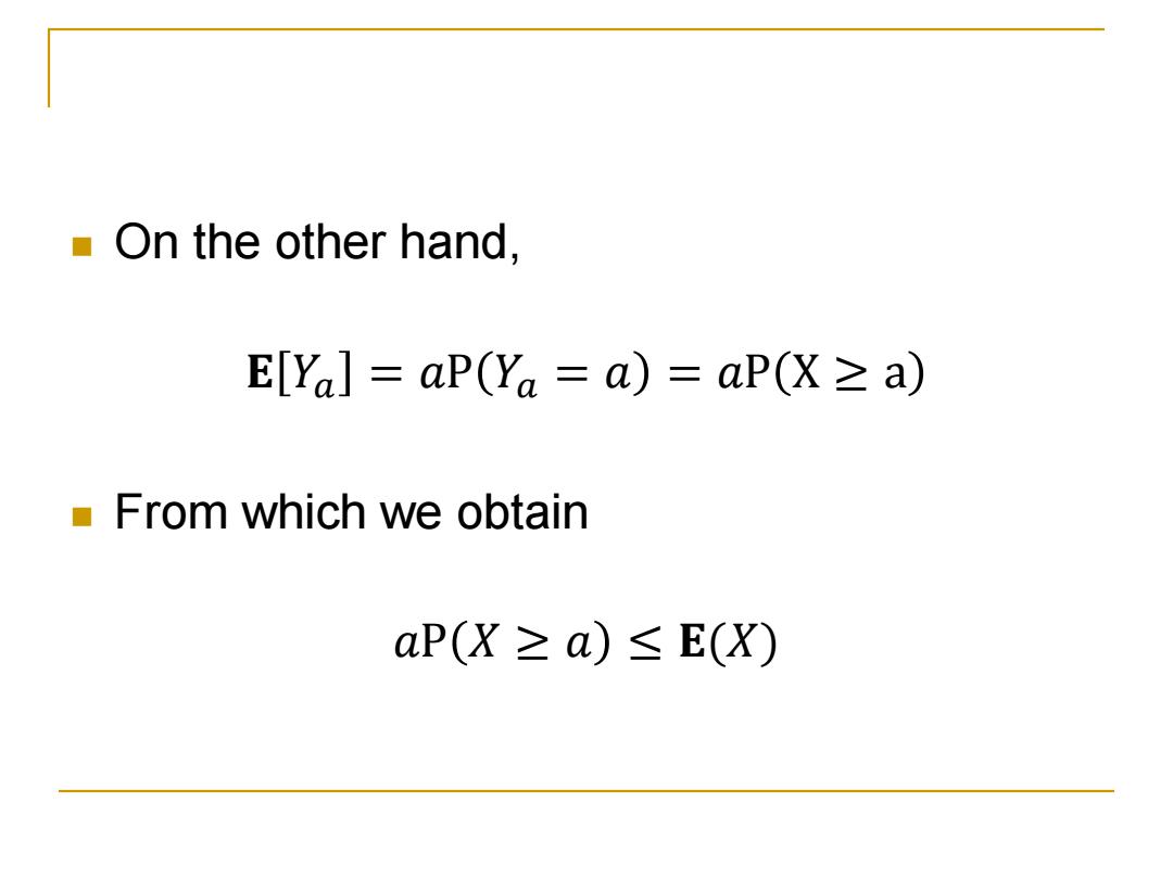
On the other hand, E[Ya]=aP(Ya =a)=aPX>a) From which we obtain aP(X≥a)≤E(X)
On the other hand, 𝐄 𝑌𝑎 = 𝑎P 𝑌𝑎 = 𝑎 = 𝑎P X ≥ a From which we obtain 𝑎P 𝑋 ≥ 𝑎 ≤ 𝐄(𝑋)
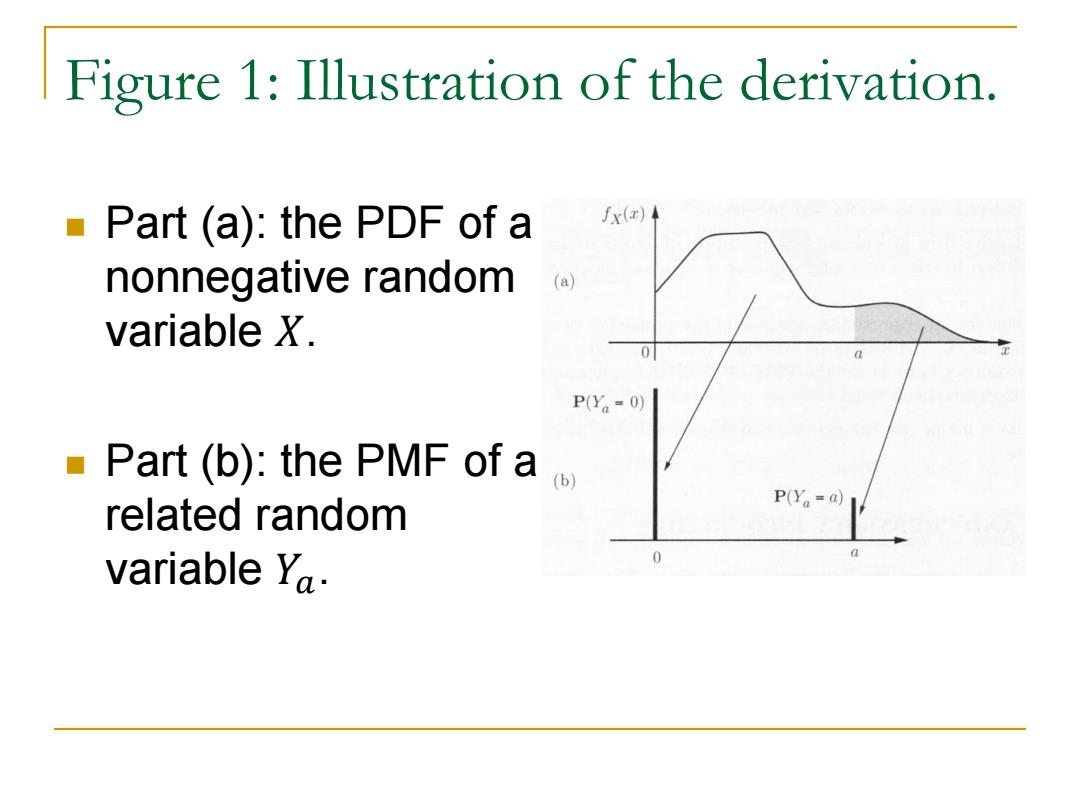
Figure 1:Illustration of the derivation. Part (a):the PDF of a fx(x) nonnegative random (a) variable X. 0 a P(Ya-0) Part (b):the PMF of a related random P(Ya=a)1 variable Ya. 0
Part (a): the PDF of a nonnegative random variable 𝑋. Part (b): the PMF of a related random variable 𝑌𝑎. Figure 1: Illustration of the derivation
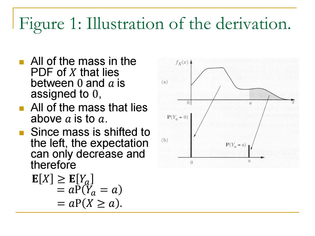
Figure 1:Illustration of the derivation. All of the mass in the fx(z) PDF of X that lies between 0 and a is (a) assigned to 0, 0 All of the mass that lies a ■ above a is to a. P(Y-0) ■ Since mass is shifted to the left,the expectation (b) P(Ya=a) can only decrease and therefore 0 E[X]≥E[Y] aP(Ya a) =aP(X≥a)
All of the mass in the PDF of 𝑋 that lies between 0 and 𝑎 is assigned to 0, All of the mass that lies above 𝑎 is to 𝑎. Since mass is shifted to the left, the expectation can only decrease and therefore 𝐄 𝑋 ≥ 𝐄 𝑌𝑎 = 𝑎P 𝑌𝑎 = 𝑎 = 𝑎P 𝑋 ≥ 𝑎 . Figure 1: Illustration of the derivation
Example 1. Let X be uniformly distributed in 0,4. Note that E[X]=2. Then,the Markov inequality asserts that 2 P(X≥2)≤ 1. P(X≥3)≤ 三 0.67. P(X≥4)≤ 二4 三 0.5
Example 1. Let 𝑋 be uniformly distributed in 0,4 . Note that 𝐄[𝑋] = 2. Then, the Markov inequality asserts that P 𝑋 ≥ 2 ≤ 2 2 = 1. P 𝑋 ≥ 3 ≤ 2 3 = 0.67. P 𝑋 ≥ 4 ≤ 2 4 = 0.5
Example 1. By comparing with the exact probabilities 2 P(X≥2)≤ 5三 P(X≥2)=0.5. 2 P(X≥3)≤ =0.67.P(X≥3)=0.25. 2 P(X≥4)≤ 4 =0.5.P(X≥4)=0. We see that the bounds provided by the Markov inequality can be quite loose
Example 1. By comparing with the exact probabilities P 𝑋 ≥ 2 ≤ 2 2 = 1. P 𝑋 ≥ 2 = 0.5. P 𝑋 ≥ 3 ≤ 2 3 = 0.67. P 𝑋 ≥ 3 = 0.25. P 𝑋 ≥ 4 ≤ 2 4 = 0.5. P 𝑋 ≥ 4 = 0. We see that the bounds provided by the Markov inequality can be quite loose