feasibility The constraints of the form ax1+bx2 =c is a line on the plane of (x1,2). (a) 400 ■ ax1+bx2≤c?half space. 30 口x1≤200 ▣ x2≤300 口 x1+x2≤400 口 X1,X2≥0 E1 100 200 300 400 All constraints are satisfied:the intersection of these half spaces.---feasible region. Feasible region nonempty:LP is feasible Feasible region empty:LP is infeasible 11
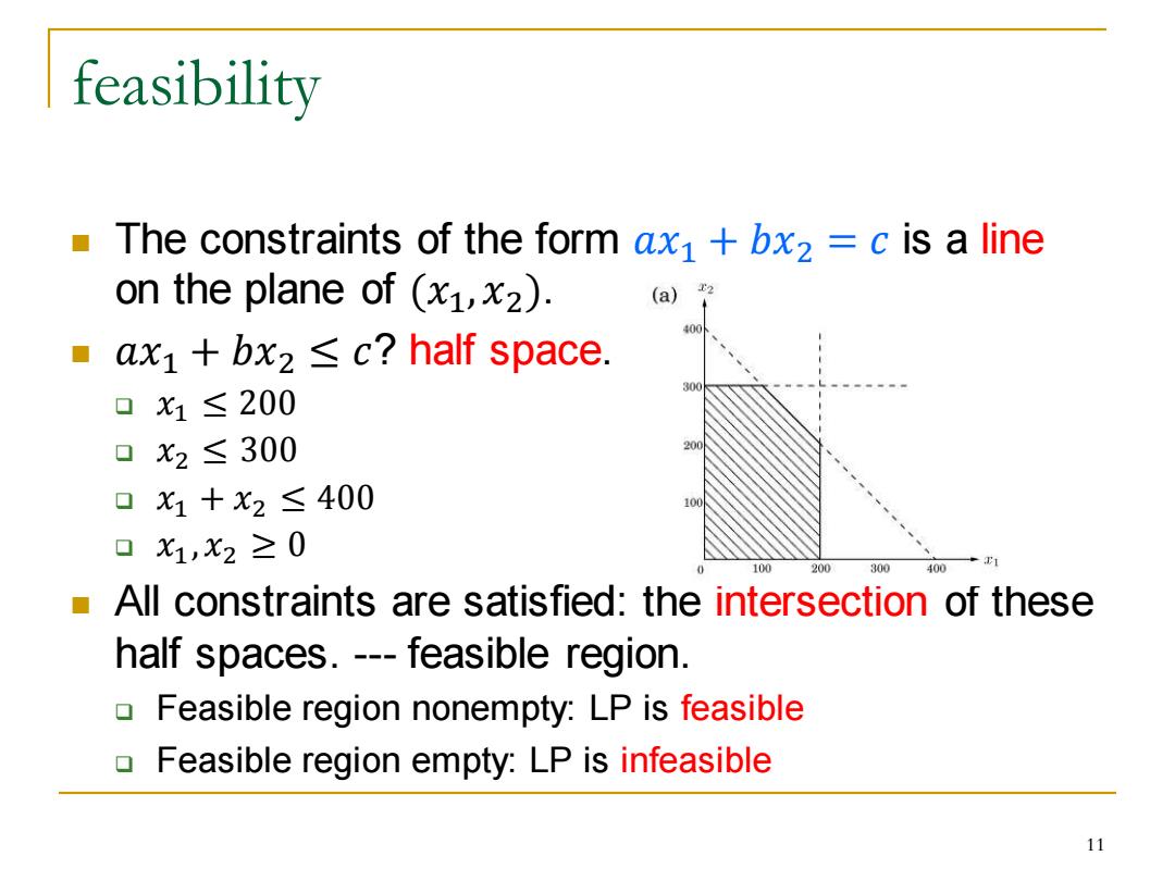
feasibility ◼ The constraints of the form 𝑎𝑥1 + 𝑏𝑥2 = 𝑐 is a line on the plane of (𝑥1, 𝑥2). ◼ 𝑎𝑥1 + 𝑏𝑥2 ≤ 𝑐? half space. ❑ 𝑥1 ≤ 200 ❑ 𝑥2 ≤ 300 ❑ 𝑥1 + 𝑥2 ≤ 400 ❑ 𝑥1, 𝑥2 ≥ 0 ◼ All constraints are satisfied: the intersection of these half spaces. --- feasible region. ❑ Feasible region nonempty: LP is feasible ❑ Feasible region empty: LP is infeasible 11
Adding the objective function into the picture The objective function is also linear (b) also a line for a fixed value. 400 Optimum point Profit $1900 Thus the optimization is: 300 try to move the line towards 200-- ----,c=1500 ----·c=1200 the desirable direction s.t. 100 ----.c=600 the line still intersects with 100 200 300 400 the feasible region. 12
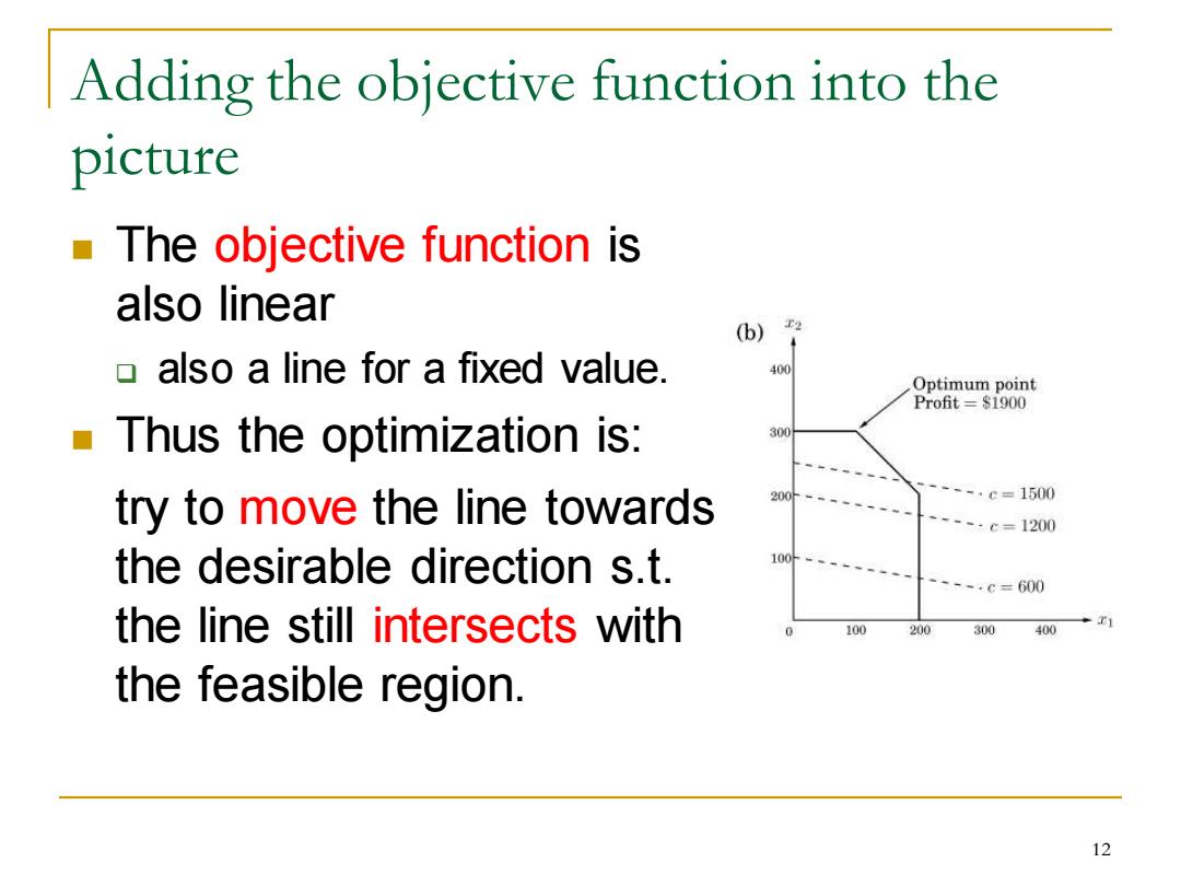
Adding the objective function into the picture ◼ The objective function is also linear ❑ also a line for a fixed value. ◼ Thus the optimization is: try to move the line towards the desirable direction s.t. the line still intersects with the feasible region. 12

Possibilities of solution Infeasible:no solution satisfying Ax=b and x≥0. Example?Picture? Feasible but unbounded:cx can be arbitrarily large. Example?Picture? Feasible and bounded:there is an optimal solution. ▣Example?Picture? 13
Possibilities of solution ◼ Infeasible: no solution satisfying 𝐴𝒙 = 𝒃 and 𝒙 ≥ 0. ❑ Example? Picture? ◼ Feasible but unbounded: 𝒄 𝑇𝒙 can be arbitrarily large. ❑ Example? Picture? ◼ Feasible and bounded: there is an optimal solution. ❑ Example? Picture? 13
Three Algorithms for LP Simplex algorithm (Dantzig,1947) Exponential in worst case Widely used due to the practical efficiency Ellipsoid algorithm (Khachiyan,1979) First polynomial-time algorithm:0(nL) L:number of input bits Weakly polynomial time Little practical impact. a Interior point algorithm (Karmarkar,1984) More efficient in theory:0(n3.5L) More efficient in practice (compared to Ellipsoid). 14
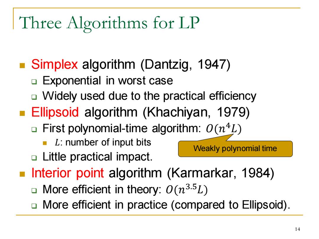
Three Algorithms for LP ◼ Simplex algorithm (Dantzig, 1947) ❑ Exponential in worst case ❑ Widely used due to the practical efficiency ◼ Ellipsoid algorithm (Khachiyan, 1979) ❑ First polynomial-time algorithm: 𝑂(𝑛 4𝐿) ◼ 𝐿: number of input bits ❑ Little practical impact. ◼ Interior point algorithm (Karmarkar, 1984) ❑ More efficient in theory: 𝑂(𝑛 3.5𝐿) ❑ More efficient in practice (compared to Ellipsoid). Weakly polynomial time 14
Simplex method:geometric view Start from any vertex of the feasible region. ■ Repeatedly look for a better neighbor and move to it. Profit $1900 300 Better:for the objective function 200 $1400 Finally we reach a point with 100 no better neighbor In other words,it's locally optimal. $0。 $200 100 200 For LP:locally optimal globally optimal. 0 Reason:the feasible region is a convex set. 15
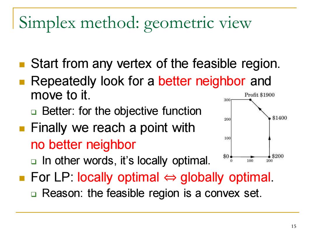
Simplex method: geometric view ◼ Start from any vertex of the feasible region. ◼ Repeatedly look for a better neighbor and move to it. ❑ Better: for the objective function ◼ Finally we reach a point with no better neighbor ❑ In other words, it’s locally optimal. ◼ For LP: locally optimal ⇔ globally optimal. ❑ Reason: the feasible region is a convex set. 15