ME369 Modeling,Analysis and System Control-A --Lecture 141112 Week 9# Nov.10(M) Frequency-Introduction,Response Ch7.1 HW4 due Nov.12(W) Frequency-Nyquist Plot Ch7.3 HW5 Week 10# Nov.17(M) Midterm Exam Nov.19(W) Frequency-Bode Diagram Ch7.2
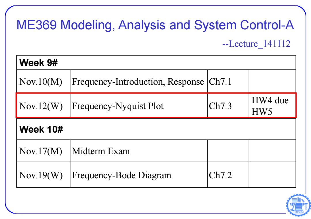
ME369 Modeling, Analysis and System Control-A --Lecture_141112 Week 9# Nov.10(M) Frequency-Introduction, Response Ch7.1 Nov.12(W) Frequency-Nyquist Plot Ch7.3 HW4 due HW5 Week 10# Nov.17(M) Midterm Exam Nov.19(W) Frequency-Bode Diagram Ch7.2

Midterm Exam announcement ·Date:Now.17(M① Time:7:50~9:50 120 minutes ·Place:Education Building D-502(东上院) One piece ofA4 paper is allowed, must be hand written
Midterm Exam announcement • Date: Nov. 17 (M) • Time: 7:50~9:50 , 120 minutes • Place: Education Building D-502 ( 东上院 ) • One piece of A4 paper is allowed, must be hand written
Problems of HW5 ·Refer to the ftp site. ftp://public.sjtu.edu.cn ·User:yuanjj ·Password:public DUE:Dec.3(W)
Problems of HW5 • Refer to the ftp site. • ftp://public.sjtu.edu.cn • User: yuanjj • Password: public DUE: Dec.3(W)
The Nyquist Plots(Polar plots) [Polar Plot]:the Nyquist plot of a sinusoidal transfer function G(j@) is a plot of the magnitude versus the phase angle in polar coordinates as w is varied from 0 to oo. Im Im U(一 0 Re 0 Re p() p(ol) A(j) p(2) A(⊙1) G(j 2) G0)
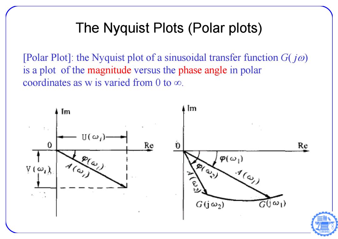
[Polar Plot]: the Nyquist plot of a sinusoidal transfer function G( j ) is a plot of the magnitude versus the phase angle in polar coordinates as w is varied from 0 to ∞. The Nyquist Plots (Polar plots)
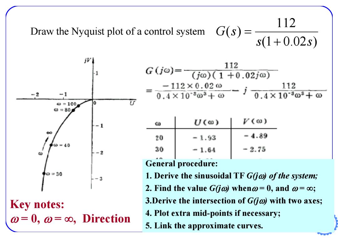
112 Draw the Nyquist plot of a control system G(S)= s(1+0.02s) 112 G(j0)=G©)(1+0.02j0) -112×0.02 2-j0.4×100+0 112 =2 -1 0.4×10803+ o=100 可 a=80f C U(@) (c) -1 00 20 -1.93 =4.89 ⊙=40 30 2 -1.64 -2.75 General procedure: 0=30 1.Derive the sinusoidal TF G@ofthe system; 2.Find the value G(@when@=0,ando=oo; Key notes: 3.Derive the intersection of G(@)with two axes; @=0,@=oo,Direction 4.Plot extra mid-points if necessary; 5.Link the approximate curves
Draw the Nyquist plot of a control system Key notes: = 0, = , Direction General procedure: 1. Derive the sinusoidal TF G(j ) of the system; 2. Find the value G(j ) when= 0, and = ; 3.Derive the intersection of G(j ) with two axes; 4. Plot extra mid-points if necessary; 5. Link the approximate curves. ( 1 0.02 ) 112 ( ) s s G s