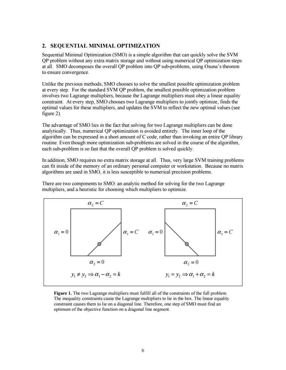
2.SEQUENTIAL MINIMAL OPTIMIZATION Sequential Minimal Optimization(SMO)is a simple algorithm that can quickly solve the SVM QP problem without any extra matrix storage and without using numerical QP optimization steps at all.SMO decomposes the overall QP problem into QP sub-problems,using Osuna's theorem to ensure convergence. Unlike the previous methods,SMO chooses to solve the smallest possible optimization problem at every step.For the standard SVM QP problem,the smallest possible optimization problem involves two Lagrange multipliers,because the Lagrange multipliers must obey a linear equality constraint.At every step,SMO chooses two Lagrange multipliers to jointly optimize,finds the optimal values for these multipliers,and updates the SVM to reflect the new optimal values(see figure 2). The advantage of SMO lies in the fact that solving for two Lagrange multipliers can be done analytically.Thus,numerical QP optimization is avoided entirely.The inner loop of the algorithm can be expressed in a short amount of C code,rather than invoking an entire QP library routine.Even though more optimization sub-problems are solved in the course of the algorithm, each sub-problem is so fast that the overall QP problem is solved quickly. In addition,SMO requires no extra matrix storage at all.Thus,very large SVM training problems can fit inside of the memory of an ordinary personal computer or workstation.Because no matrix algorithms are used in SMO,it is less susceptible to numerical precision problems. There are two components to SMO:an analytic method for solving for the two Lagrange multipliers,and a heuristic for choosing which multipliers to optimize. a,=C a,=C a1=0 a=C 0x1=0 =C 02=0 x2=0 y≠y3→0x1-02=k 片=2→01+0x2=k Figure 1.The two Lagrange multipliers must fulfill all of the constraints of the full problem. The inequality constraints cause the Lagrange multipliers to lie in the box.The linear equality constraint causes them to lie on a diagonal line.Therefore,one step of SMO must find an optimum of the objective function on a diagonal line segment. 6
6 2. SEQUENTIAL MINIMAL OPTIMIZATION Sequential Minimal Optimization (SMO) is a simple algorithm that can quickly solve the SVM QP problem without any extra matrix storage and without using numerical QP optimization steps at all. SMO decomposes the overall QP problem into QP sub-problems, using Osuna’s theorem to ensure convergence. Unlike the previous methods, SMO chooses to solve the smallest possible optimization problem at every step. For the standard SVM QP problem, the smallest possible optimization problem involves two Lagrange multipliers, because the Lagrange multipliers must obey a linear equality constraint. At every step, SMO chooses two Lagrange multipliers to jointly optimize, finds the optimal values for these multipliers, and updates the SVM to reflect the new optimal values (see figure 2). The advantage of SMO lies in the fact that solving for two Lagrange multipliers can be done analytically. Thus, numerical QP optimization is avoided entirely. The inner loop of the algorithm can be expressed in a short amount of C code, rather than invoking an entire QP library routine. Even though more optimization sub-problems are solved in the course of the algorithm, each sub-problem is so fast that the overall QP problem is solved quickly. In addition, SMO requires no extra matrix storage at all. Thus, very large SVM training problems can fit inside of the memory of an ordinary personal computer or workstation. Because no matrix algorithms are used in SMO, it is less susceptible to numerical precision problems. There are two components to SMO: an analytic method for solving for the two Lagrange multipliers, and a heuristic for choosing which multipliers to optimize. Figure 1. The two Lagrange multipliers must fulfill all of the constraints of the full problem. The inequality constraints cause the Lagrange multipliers to lie in the box. The linear equality constraint causes them to lie on a diagonal line. Therefore, one step of SMO must find an optimum of the objective function on a diagonal line segment. a2 = C a2 = C a2 = 0 a1 = 0 a1 = C yy k 12 12 ¡Æ- = a a a2 = 0 a1 = 0 a1 = C yy k 12 12 =Æ+ = a a
2.1 Solving for Two Lagrange Multipliers In order to solve for the two Lagrange multipliers,SMO first computes the constraints on these multipliers and then solves for the constrained minimum.For convenience,all quantities that refer to the first multiplier will have a subscript 1,while all quantities that refer to the second multiplier will have a subscript 2.Because there are only two multipliers,the constraints can be easily be displayed in two dimensions(see figure 3).The bound constraints(9)cause the Lagrange multipliers to lie within a box,while the linear equality constraint(6)causes the Lagrange multipliers to lie on a diagonal line.Thus,the constrained minimum of the objective function must lie on a diagonal line segment(as shown in figure 3).This constraint explains why two is the minimum number of Lagrange multipliers that can be optimized:if SMO optimized only one multiplier,it could not fulfill the linear equality constraint at every step. The ends of the diagonal line segment can be expressed quite simply.Without loss of generality, the algorithm first computes the second Lagrange multiplier o and computes the ends of the diagonal line segment in terms of o2.If the target yi does not equal the target y2,then the following bounds apply to L=max(0,a,-a),H=min(C,C+a2). (13) If the target y equals the target y2,then the following bounds apply to L=max(0,a,+a-C),H=min(C,a,+a) (14) The second derivative of the objective function along the diagonal line can be expressed as: n=K(1,x1)+K(2,x2)-2K(1,x2) (15) Under normal circumstances,the objective function will be positive definite,there will be a minimum along the direction of the linear equality constraint,and n will be greater than zero.In this case,SMO computes the minimum along the direction of the constraint: "=g+2(E-E2) (16) n where E,=u,-y,is the error on the ith training example.As a next step,the constrained minimum is found by clipping the unconstrained minimum to the ends of the line segment: H if anew≥H; w.clipped if L<ag<H (17) L if ew≤L. Now,let s=yy2.The value of o is computed from the new,clipped,2: aew=a+s(a-awcipped ) (18) Under unusual circumstances,n will not be positive.A negative n will occur if the kernel K does not obey Mercer's condition,which can cause the objective function to become indefinite.A zero n can occur even with a correct kernel,if more than one training example has the same input >
7 2.1 Solving for Two Lagrange Multipliers In order to solve for the two Lagrange multipliers, SMO first computes the constraints on these multipliers and then solves for the constrained minimum. For convenience, all quantities that refer to the first multiplier will have a subscript 1, while all quantities that refer to the second multiplier will have a subscript 2. Because there are only two multipliers, the constraints can be easily be displayed in two dimensions (see figure 3). The bound constraints (9) cause the Lagrange multipliers to lie within a box, while the linear equality constraint (6) causes the Lagrange multipliers to lie on a diagonal line. Thus, the constrained minimum of the objective function must lie on a diagonal line segment (as shown in figure 3). This constraint explains why two is the minimum number of Lagrange multipliers that can be optimized: if SMO optimized only one multiplier, it could not fulfill the linear equality constraint at every step. The ends of the diagonal line segment can be expressed quite simply. Without loss of generality, the algorithm first computes the second Lagrange multiplier α2 and computes the ends of the diagonal line segment in terms of α2. If the target y1 does not equal the target y2, then the following bounds apply to α2: L H = − = +− max( , ), 0 α 21 21 α min(C, ). C α α (13) If the target y1 equals the target y2, then the following bounds apply to α2: L = +− = + max( , ), min( , ). 0 α 21 21 α C H C α α (14) The second derivative of the objective function along the diagonal line can be expressed as: η =+− Kx x Kx x Kx x ( , ) ( , ) ( , ). rr rr rr 11 2 2 12 2 (15) Under normal circumstances, the objective function will be positive definite, there will be a minimum along the direction of the linear equality constraint, and η will be greater than zero. In this case, SMO computes the minimum along the direction of the constraint : α α η 2 2 new 21 2 = + yE E ( ) − , (16) where E u y iii = - is the error on the ith training example. As a next step, the constrained minimum is found by clipping the unconstrained minimum to the ends of the line segment: α α α α α 2 2 2 2 2 new,clipped new new new new if if L if = ≥ < < ≤ % & K ' K H H L H L ; ; . (17) Now, let s yy = 1 2 . The value of α1 is computed from the new, clipped, α2: α 1 1 22 α α α new new,clipped =+ − s( ). (18) Under unusual circumstances, η will not be positive. A negative η will occur if the kernel K does not obey Mercer’s condition, which can cause the objective function to become indefinite. A zero η can occur even with a correct kernel, if more than one training example has the same input